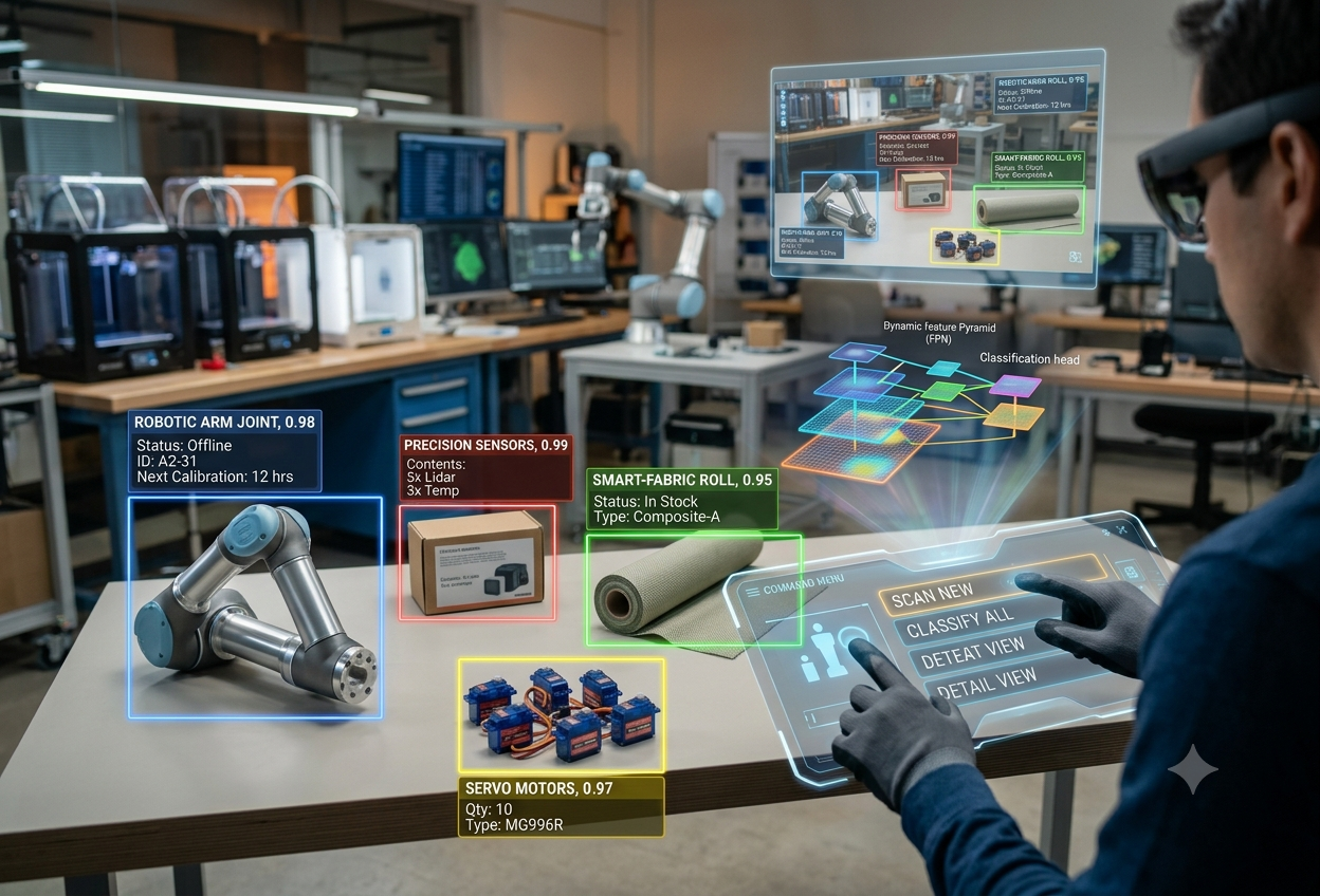
Object Detection
What Is Object Detection?
Close your eyes for a second and picture your kitchen table. Without even trying, your brain instantly knows that there is a mug here, an apple there, and a phone near the edge — and it knows exactly where each one sits. Object detection is the branch of artificial intelligence that teaches a computer to do that same trick with a photograph or a video frame.
Object detection is the computer-vision task of finding every object that belongs to a chosen category inside an image, drawing a tight box around each one, and naming what it is — all at the same time.— Working Definition Used Throughout This Guide
That single sentence hides two separate jobs that the computer must do together. The first job is localisation — figuring out exactly where an object sits in the picture, usually by drawing a rectangle, called a bounding box, around it. The second job is classification — deciding what category that object belongs to, such as “car,” “dog,” or “traffic light.” A model only counts as a true object detector when it can do both jobs, for every object, in a single image, at the same time.
Imagine you are playing “I Spy” with a magic pair of glasses. The glasses do not just say “I spy something” — they draw a little box around every single thing they spot and whisper its name in your ear: “box around the cat, box around the ball, box around the shoe.” That is exactly what an object detection program does to a picture, except it never gets tired and it can do it thousands of times a second.
Object Detection vs. Its Close Cousins
People often mix up object detection with three related computer-vision tasks. They are all about “looking” at an image, but each one answers a slightly different question, and mixing them up can lead to picking the wrong tool for a project.
Looks at the whole picture and gives it one label, such as “this photo contains a dog.” It never says where the dog is or how many dogs there are.
What?Finds the position of one main object in a picture and draws a single box around it, but does not try to find every object or label its category in detail.
Where?Combines the two jobs above for every object of interest in the image at once — multiple boxes, multiple labels, one pass over the picture.
What & Where?Goes one step further than detection by colouring in the exact pixels that belong to each object instead of just drawing a rectangular box around it.
Exact ShapeWhat a Bounding Box Actually Is
A bounding box is simply the smallest rectangle that can fully wrap around an object without cutting off any part of it. Underneath the friendly rectangle on screen, the computer stores it as four numbers — usually the coordinates of the top-left corner together with a width and a height, or sometimes the coordinates of two opposite corners. Alongside the box, the model also outputs a class label (the name of the object) and a confidence score, which is a percentage that tells you how sure the model is that the box really contains that object.
A Quick Word on Confidence Scores
Whenever you see a percentage next to a detected object, that number is not a guarantee — it is the model’s own estimate of how likely it is that the box and the label are both correct. A confidence score of 0.97 for “car” means the model is very sure; a score of 0.40 means it is only somewhat sure, and many systems are configured to throw away anything below a chosen threshold so the final output only shows detections the model genuinely trusts.
Why Object Detection Matters So Much
Object detection is one of the most fundamental building blocks in computer vision because so many other intelligent behaviours depend on it first knowing what is in front of it and exactly where. It is the sensory layer that lets a machine react to the world instead of just describing it.
Think about everything a self-driving car has to do in a single second: it must notice the pedestrian stepping off the curb, the cyclist weaving between lanes, the traffic light turning amber, and the delivery van braking ahead — and it must know precisely where each of those things is so it can steer, brake, or accelerate correctly. A plain image classifier that only says “this scene contains a pedestrian” would be almost useless here, because the car also needs to know exactly where that pedestrian is standing relative to its own wheels. This is exactly the gap that object detection fills, and it is why the technique sits underneath so many other computer-vision systems, including tracking, captioning, and pose estimation.
Imagine trying to cross a busy road wearing a blindfold, but someone shouts “there’s a car!” without telling you which direction or how far away. That warning is not very useful, is it? Now imagine they shout “car, ten steps to your left, coming closer!” Suddenly you can actually do something about it. Object detection gives computers that second, much more useful kind of warning.
From One Decision a Day to Millions a Second
Fifty years ago, “spotting an object correctly” was a job done entirely by trained human eyes — a radiologist studying one X-ray at a time, or a security guard watching one camera feed. Today, a single trained object detection model can be copied onto thousands of cameras, cars, or scanners simultaneously, each one making the same kind of decision dozens of times every second. That is not just a speed improvement; it is a completely different scale of operation, and it is part of why getting object detection right — and getting it to fail safely when it is wrong — matters so much for industries like healthcare, transport, and security.
It Is a Building Block, Not Just an End Product
In most real systems, object detection is rarely the final goal on its own — it is the first link in a longer chain. Once a car or a person is detected and boxed in one video frame, a separate tracking algorithm can follow that same box across many frames to understand movement and speed. Once a tumour-like region is detected on a scan, a doctor can zoom in for a closer look. Once a product is detected on a store shelf, an inventory system can update its stock count automatically. Object detection is the doorway through which a huge share of practical AI applications must first pass.
Because object detection often feeds directly into automated decisions, an error is not just an academic statistic — it can mean a security system missing an unattended bag, a factory line failing to flag a damaged part, or a driver-assistance feature reacting a moment too late to a pedestrian. This is precisely why so much engineering effort, covered later in this guide, goes into measuring detection quality carefully and stress-testing models against tricky real-world conditions before they are deployed.
How Object Detection Works: The Pipeline
Even though dozens of different object detection architectures exist, almost every modern deep-learning detector is built from the same three-part skeleton: a backbone, a neck, and a head. Understanding these three parts is the single most useful mental model for making sense of everything else in this guide.
Step 1 — Turning a Picture Into Numbers
Before any “intelligence” happens, the input image first has to be prepared. A photo is really just a giant grid of tiny coloured squares called pixels, and each pixel is stored as a handful of numbers describing its colour. The image is usually resized to a fixed size and its pixel values are rescaled into a consistent numeric range, a step called normalisation, so that the neural network always receives data in a predictable shape no matter what camera or resolution the photo originally came from.
Step 2 — The Backbone: Finding Visual Features
The resized image is then fed into the backbone, a deep convolutional neural network (CNN) whose only job is to spot useful visual patterns. Small filters slide across the image looking for simple things first — edges, corners, blobs of colour — in the earliest layers. As the data moves deeper into the network, those simple patterns are combined into more complex ones, such as wheels, fur textures, or window shapes, until the network has built up a rich numerical summary of “what kind of stuff is where” in the picture. These summaries are called feature maps, and a backbone usually produces several of them at different resolutions.
Step 3 — The Neck: Mixing Information Across Scales
A small object, like a distant bird, and a large object, like a nearby truck, naturally show up most clearly at different feature-map resolutions. The neck of the network exists to fuse information across these different scales, so that the parts of the network responsible for making the final predictions have access to both fine, detailed information and broad, contextual information at the same time. A feature pyramid network is one of the most widely used neck designs for this job.
Step 4 — The Head: Predicting Boxes and Classes
Finally, the head takes the fused feature maps and produces the actual predictions. At every one of many candidate positions across the image — often guided by reference shapes called anchor boxes, which are pre-set rectangles of different sizes and aspect ratios tiled across the picture — the head predicts two things: how the position and size of that anchor should be nudged to fit a real object tightly (bounding-box regression), and how likely it is that the box belongs to each possible category (classification).
Step 5 — Cleaning Up With Non-Maximum Suppression
A single real object is almost always proposed many times over by slightly overlapping anchors, which would otherwise leave the final image cluttered with duplicate boxes around the same dog or car. A filtering step called Non-Maximum Suppression (NMS) solves this: it keeps the highest-confidence box for an object, throws away any other box that overlaps it too heavily, and repeats this process until only one clean box remains per real object.
Think of the backbone like a detective squinting at clues, the neck like an assistant who organises those clues at different zoom levels, and the head like the detective finally announcing “I’m 97% sure that’s a dog, and it’s standing right here.” The clean-up step at the end is like a teacher collecting twenty almost-identical answer sheets from group work and only keeping the best one from each group.
How Computers Detected Objects Before Neural Networks
Object detection did not begin with deep learning. For more than a decade before convolutional neural networks took over, researchers had to hand-design the rules a computer would use to recognise an object — a slow, painstaking process that nonetheless laid the groundwork for everything that followed.
The Sliding-Window Idea
One of the earliest strategies was beautifully simple: slide a fixed-size window across every possible position and scale in the image, and at each stop, ask a separate classifier “is there an object of interest inside this little box right now?” To catch objects of different sizes, the same sliding process had to be repeated on multiple resized copies of the image, which made the whole approach extremely slow on the computing hardware available at the time.
Hand-Engineered Features
Because computers could not yet learn visual patterns on their own, researchers designed mathematical recipes, called features, that turned a patch of pixels into a list of numbers describing things like edge direction or texture. A handful of these techniques became famous building blocks of early computer vision.
Used simple Haar-like patterns of light and dark rectangles to spot faces extremely quickly, making it one of the first detectors fast enough to run in something close to real time.
Measured the direction that brightness changes in small patches of an image, capturing the rough outline or silhouette of an object — famously effective for spotting pedestrians.
Found distinctive “keypoints” in an image that stayed recognisable even if the picture was rotated, resized, or the lighting changed, useful for matching the same object across photos.
Represented an object as a collection of smaller parts that could shift relative to one another, helping detectors cope with objects bending or posing in different ways.
Once a hand-crafted feature was computed, a separate, simpler machine-learning model — most often a Support Vector Machine (SVM) — was trained to decide whether those numbers represented the object being searched for. This pairing of “hand-built features plus a classical classifier” was the standard recipe for object detection for well over a decade.
Hand-crafted features had to be redesigned almost from scratch for every new object category, every lighting condition, and every camera angle, because the humans who designed them could not anticipate every possible variation in the real world. They also struggled badly with cluttered backgrounds, partial occlusion, and objects of unusual shapes or sizes. This rigidity is precisely the gap that deep learning, with its ability to learn features automatically from data rather than have them hand-designed, was able to close starting in 2014.
A Brief History of Object Detection
Object detection research is often divided into two distinct eras: a traditional era built on hand-crafted features, and a deep-learning era that began in 2014 and has been accelerating ever since.
Viola-Jones Detector
One of the first practical real-time object detectors, originally built to find human faces using fast Haar-like feature cascades.
HOG Detector
Introduced gradient-orientation features that became especially popular for pedestrian detection in surveillance and early driver-assistance research.
Deformable Part Models
Brought bounding-box regression into the mainstream and modelled objects as flexible arrangements of smaller parts.
R-CNN — Deep Learning Arrives
The first widely successful deep-learning detector; combined external region proposals with a CNN for feature extraction, kicking off the modern era.
Fast R-CNN & Faster R-CNN
Replaced slow, repeated CNN passes with a single shared computation and an internal Region Proposal Network, dramatically improving speed and accuracy.
YOLO & SSD — One-Stage Detectors
Reframed detection as a single direct prediction problem rather than two separate stages, unlocking real-time speeds for the first time.
RetinaNet & Mask R-CNN
RetinaNet’s Focal Loss closed much of the accuracy gap for one-stage detectors, while Mask R-CNN extended Faster R-CNN to also output pixel-level masks.
YOLOv3 Through YOLOv7
A rapid run of community-driven YOLO releases, each squeezing out more speed and accuracy for real-time and edge-device deployment.
DETR — Transformers Arrive
Reframed detection as a direct set-prediction problem solved by an encoder-decoder transformer, removing the need for hand-designed anchor boxes.
YOLOv8 Onward, RT-DETR, Foundation Models
Newer YOLO generations, real-time transformer detectors, and open-vocabulary, prompt-driven “detect anything” foundation models continue to push speed and flexibility further.
If you think of object detection like a video game character levelling up, the early “traditional” years were like a character with very basic, hand-picked moves. The year 2014 was a huge level-up — the character suddenly learned to teach itself new moves by watching thousands of examples, and it has kept getting faster and smarter in every level since.
One-Stage vs. Two-Stage Detectors
Nearly every deep-learning object detector falls into one of two architectural families, and the difference between them comes down to a single design choice: does the model propose candidate regions first and classify them afterward, or does it predict everything in one single pass?
Two-Stage Detectors: Look Twice, Decide Carefully
A two-stage detector first runs a lightweight network, often called a Region Proposal Network (RPN), that scans the image and suggests a smaller set of regions that probably contain something interesting. A second, more careful network then looks only at those proposed regions to decide the exact class and to fine-tune the bounding box. Splitting the work this way tends to produce very accurate, tightly fitted boxes, at the cost of extra computation and slower processing.
One-Stage Detectors: Predict Everything At Once
A one-stage detector skips the separate proposal step entirely. It treats the whole image as a dense grid of candidate positions and predicts a class and a bounding box for every position in a single forward pass through the network. This makes one-stage detectors significantly faster and simpler to deploy, which is why they dominate real-time applications such as live video analysis, though they historically traded away a little accuracy, especially on small or tightly packed objects.
| Detector Type | Strengths | Trade-Offs | Well-Known Examples |
|---|---|---|---|
| Two-Stage | High accuracy, precise box fit, fewer false alarms, easy to extend (e.g. adding segmentation masks) | Slower inference, more complex to train and tune, heavier compute and memory needs | R-CNN, Fast R-CNN, Faster R-CNN, Mask R-CNN |
| One-Stage | Real-time speed, simpler end-to-end design, well suited to mobile and edge devices | Historically weaker on small or densely packed objects, can produce more false positives | YOLO family, SSD, RetinaNet |
A two-stage detector is like a careful shopper who first walks around picking out a few promising items, then goes back to inspect each one closely before buying. A one-stage detector is like a shopper who glances at the whole shelf once and grabs everything that looks right immediately — much faster, but occasionally grabs the wrong thing by mistake.
Popular Object Detection Algorithms & Models
Dozens of named architectures have been published since 2014, but most of them are variations on a handful of core ideas. This section walks through the families that every working engineer is likely to encounter.
The R-CNN Family — Two-Stage Pioneers
The original R-CNN (Region-based Convolutional Neural Network), introduced in 2014, generated roughly two thousand candidate regions per image using a separate, non-learned algorithm, then ran each region through a CNN to extract features before classifying it with a support vector machine. It worked remarkably well for its time but was painfully slow, because the CNN had to process thousands of regions one by one for every single image.
Fast R-CNN (2015) fixed the worst of this by running the CNN only once over the entire image and then pooling features for each region of interest from that single shared feature map, dramatically cutting training and inference time. Faster R-CNN (2015) went a step further by replacing the external region-proposal algorithm with an internal, learnable Region Proposal Network that shares the same backbone as the rest of the network, allowing the whole system to be trained end-to-end. Mask R-CNN (2017) then extended Faster R-CNN with an extra branch that predicts a pixel-level mask for every detected object, effectively combining object detection with instance segmentation in a single model.
The YOLO Family — Built for Speed
YOLO (You Only Look Once), first released in 2016, took a radically different approach: instead of proposing and then classifying regions, it divides the image into a grid and asks each grid cell to directly predict a small number of bounding boxes and class probabilities in a single forward pass. This condenses the entire pipeline into one network, making YOLO dramatically faster than the R-CNN family and a favourite for real-time use cases such as live video and robotics.
The YOLO lineage has been updated almost every year since, with each generation tightening the trade-off between speed and accuracy. Later versions introduced techniques such as cross-stage partial connections for more efficient backbones, multi-scale feature fusion in the neck, dynamic training strategies that remove the need for a separate non-maximum-suppression step at inference time, and lightweight “nano” variants designed specifically to run on phones, drones, and other edge devices.
SSD and RetinaNet — Other One-Stage Approaches
The Single Shot MultiBox Detector (SSD), also released in 2016, predicts boxes and class scores directly from several feature maps taken at different layers of the backbone network, letting smaller feature maps watch for larger objects and larger feature maps watch for smaller ones. RetinaNet (2017) tackled a different problem common to one-stage detectors: because the vast majority of grid positions in any image contain only background, training can be swamped by easy negative examples. RetinaNet introduced a technique called Focal Loss, which automatically down-weights the contribution of easy, already well-classified examples so that training pays more attention to the harder, more informative ones — helping one-stage detectors close much of the accuracy gap with their two-stage cousins.
Transformer-Based Detectors
Around 2020, the same self-attention mechanism that had transformed natural language processing began making its way into computer vision. DETR (DEtection TRansformer) reframed object detection as a direct set-prediction problem: a convolutional backbone extracts features, and an encoder-decoder transformer then predicts a fixed set of boxes and classes directly, with a clever matching algorithm pairing each prediction to a real object during training. This elegantly removed the need for hand-designed anchor boxes and the separate non-maximum-suppression step altogether. Later transformer-based detectors, including real-time variants, have continued to narrow the speed gap with CNN-based models while keeping the flexibility that self-attention provides for capturing relationships across the whole image rather than just nearby pixels.
| Model Family | Year Introduced | Core Idea | Best Known For |
|---|---|---|---|
| R-CNN | 2014 | External region proposals + CNN features + SVM classifier | Kick-starting the deep-learning era of detection |
| Fast / Faster R-CNN | 2015 | Shared CNN pass + learnable Region Proposal Network | Strong accuracy baseline, end-to-end training |
| YOLO Family | 2016 – present | Single-pass grid prediction of boxes and classes | Real-time speed, edge and mobile deployment |
| SSD | 2016 | Multi-scale feature maps for direct box prediction | Simple, easy-to-integrate one-stage detector |
| RetinaNet | 2017 | Focal Loss to fix class imbalance in one-stage training | Closing the accuracy gap for one-stage models |
| Mask R-CNN | 2017 | Faster R-CNN + a parallel pixel-mask branch | Combined detection and instance segmentation |
| DETR & Successors | 2020 – present | Transformer-based direct set prediction | Removing anchors and NMS, global context |
R-CNN is like a student who carefully re-reads every paragraph of a book before answering a question — accurate, but slow. YOLO is like a student who skims the whole page once and answers immediately — much faster, and surprisingly good at getting the right answer. Transformer-based models are like a student who can pay attention to every single word in the whole book at once, no matter how far apart those words are.
How Object Detection Models Are Evaluated
A model that just says “yes, there’s a dog somewhere” is not very useful if its box is nowhere near the actual dog. Object detection therefore needs evaluation metrics that judge both the location and the label of a prediction together, and a handful of standard metrics have become the common language researchers and engineers use to compare models fairly.
Intersection over Union (IoU)
IoU is the foundation that almost every other detection metric is built on top of. It measures how well a predicted box overlaps with the true, human-labelled “ground truth” box, by dividing the area where the two boxes overlap by the total area the two boxes cover together. A perfect match scores 1.0; two boxes that do not touch at all score 0.
Precision and Recall
Once IoU decides whether a single predicted box counts as a correct “true positive” match (commonly using an IoU threshold such as 0.5), two classic information-retrieval metrics take over to summarise overall performance. Precision answers the question “of everything the model said was an object, how much did it actually get right?” Recall answers the opposite question, “of all the real objects that existed in the image, how many did the model actually manage to find?” A model can score perfectly on one of these by cheating in a lazy way — for example, predicting almost nothing gives very high precision but terrible recall — which is exactly why neither metric is trusted alone.
Average Precision (AP) and Mean Average Precision (mAP)
To capture the trade-off between precision and recall properly, researchers plot a precision-recall curve as the model’s confidence threshold is varied, and then measure the area under that curve for a single object class — this is the Average Precision (AP) for that class. Averaging the AP across every category in the dataset produces the single most widely reported object detection metric of all: mean Average Precision (mAP). A higher mAP means a model is, on balance, doing a better job of finding objects accurately and confidently across every category it was trained on.
Speed Metrics: FPS and Inference Time
Accuracy alone does not tell the whole story, especially for applications like autonomous driving or live video analytics where a model has only a fraction of a second to make a decision. Frames Per Second (FPS) measures how many images a model can process every second, and inference time measures how many milliseconds a single image takes to process — the two are simply each other’s reciprocal. Choosing a model is almost always a balancing act between mAP and FPS, since the most accurate models are rarely the fastest ones.
Overlap between predicted and true box. The building block every other metric depends on.
Of the model’s positive predictions, what fraction were actually correct?
Of all the real objects present, what fraction did the model successfully find?
The average “AP” score across every object class — the headline benchmark number.
Imagine a treasure hunt where you have to both find hidden coins and point exactly to where each one is buried. Precision asks, “of the spots you dug, how many actually had a coin?” Recall asks, “of all the real coins buried, how many did you actually dig up?” A good treasure hunter — and a good object detector — needs to score well on both at the same time, not just one.
Datasets That Power Object Detection
A detection model can only ever be as good as the labelled examples it was trained on. Building a useful dataset means collecting thousands of images and patiently drawing a bounding box and a category label around every object of interest in each one — a process called annotation, which is often the single most expensive and time-consuming part of building a real-world detection system.
The Benchmark Datasets Everyone Refers To
MS COCO
Common Objects in Context — a widely used benchmark covering 80 everyday object categories across hundreds of thousands of richly annotated images, used to compare almost every modern detector’s mAP score.
Pascal VOC
One of the original standard benchmarks for object detection research, with twenty object categories; still widely used in tutorials and academic comparisons today.
ImageNet
Best known for image classification, but its backbone networks — pretrained on its millions of labelled images — are reused as the starting point for countless detection models.
Open Images & LVIS
Open Images offers millions of images across thousands of categories; LVIS specifically focuses on the long tail of rare object categories that ordinary datasets barely cover.
Why Annotation Quality Decides Everything
An object detection model learns its entire sense of “what counts as a correct box” purely from the examples humans gave it — so a dataset with sloppy, inconsistent, or biased boxes will quietly teach the model the same sloppiness, inconsistency, or bias. Specialised annotation tools and platforms exist purely to make this labelling process faster, more consistent, and easier to manage across large teams of human annotators.
Stretching Limited Data Further
Because gathering and labelling enough images is expensive, practitioners lean on three complementary techniques to make the most of what they have. Transfer learning starts from a backbone already pretrained on a huge general dataset like ImageNet or COCO, so the model only needs to fine-tune on a much smaller, task-specific dataset rather than learning to see from zero. Data augmentation artificially multiplies the training set by flipping, rotating, cropping, recolouring, or even combining multiple images together, teaching the model to recognise objects under variations it has not literally seen before. Active learning flips the usual labelling order around: instead of randomly choosing which images to label next, the model itself flags the images it is currently most uncertain about, so human effort gets spent labelling exactly the examples that will teach the model the most.
Training a detector without a good dataset is like trying to learn what a “fair” referee call looks like by only ever watching one team’s matches — you would end up with a very lopsided idea of fairness. The bigger and more varied the set of pictures a model studies, the fairer and more reliable its judgement becomes once it meets brand-new pictures it has never seen before.
Where Object Detection Shows Up in Everyday Life
Object detection has quietly become one of the most widely deployed pieces of artificial intelligence in the world, sitting inside products and systems that millions of people interact with every single day, often without realising a detector is running at all.
Autonomous & Assisted Driving
Self-driving systems and driver-assistance features rely on object detection to spot pedestrians, cyclists, other vehicles, traffic signs, and lane markings in real time, feeding that information directly into steering and braking decisions.
Medical Imaging
Detectors help highlight possible tumours, lesions, or other abnormalities on X-rays, CT scans, and MRIs, drawing a radiologist’s attention to the regions most worth a closer look without replacing their final judgement.
Security & Surveillance
Camera networks use detection to flag intruders in restricted areas, unattended bags, or unusual crowd behaviour, alerting human operators instead of requiring someone to watch every single feed at once.
Retail & Inventory
Smart shelves and checkout-free stores detect which products a shopper picks up, while warehouse systems use detection to count stock and flag empty or misplaced items automatically.
Agriculture
Drones and field cameras detect ripe fruit, diseased crops, weeds, or livestock, helping farmers act on precise, localised information rather than guessing across an entire field.
Manufacturing
Production-line cameras detect scratches, dents, or missing components on products moving past at speed, catching defects far more consistently than a tired human eye on a long shift.
Aerial & Satellite Imagery
Detection applied to drone and satellite photos helps spot buildings, vehicles, or storm damage across huge areas — useful for urban planning, disaster response, and environmental monitoring.
Document Analysis
Beyond photographs, detection also locates tables, signatures, and text blocks within scanned documents, automating tasks like invoice processing and form data extraction.
Wherever a system needs to know not just what is in front of it, but exactly where, an object detector is usually doing the looking.
— Recurring Theme Across Modern Computer-Vision PracticePros & Cons of Object Detection
Object detection is a genuinely powerful tool, but like every technology it comes with real trade-offs that are worth understanding honestly before relying on it for an important decision.
Strengths
- Finds and labels many objects in one pass, far faster than manual review
- Works continuously, around the clock, without losing attention
- Scales to thousands of cameras or images at once after training only one model
- Modern lightweight versions run on phones, drones, and other small devices
- Provides precise location data, not just a vague “object present” label
Limitations
- Accuracy depends heavily on image quality, lighting, and camera angle
- Struggles with heavily occluded, very small, or oddly posed objects
- Needs large amounts of carefully labelled training data to perform well
- High-accuracy models can be computationally expensive to run at scale
- Only draws a box, not an exact outline — segmentation is needed for pixel-level precision
Object Detection vs. Image Segmentation: Which One Do You Actually Need?
Because a bounding box is rectangular, it always includes a little bit of background along with the object, and it cannot capture an unusual or irregular shape precisely. For tasks where that imprecision genuinely matters — measuring the exact area of a tumour, or guiding a robotic arm around an irregular part — engineers often reach for instance segmentation instead, which is more computationally expensive but draws a pixel-accurate outline rather than a simple box. For most everyday tasks, though, a bounding box is more than precise enough, and it comes at a fraction of the computational cost.
Object detection is best understood as a powerful pattern-matching tool, not a system that truly “understands” objects the way a person does. A model recognises a pattern of pixels that resembled “pedestrian” in its training data — it does not know what a pedestrian is, why they might step into the road, or how to reason about a genuinely novel situation it has never encountered before. Keeping this limitation in mind is essential whenever object detection feeds into a safety-critical decision.
Challenges in Object Detection
Despite two decades of rapid progress, object detection is far from a solved problem. Several stubborn challenges keep researchers and engineers busy, and understanding them helps explain why detectors sometimes fail in ways that seem obvious to a human observer.
The same kind of object can appear tiny in the distance or huge up close within a single image, and a model must recognise it confidently at every size.
Objects are often partly hidden behind something else — a person behind a car, a product behind another product — leaving the model with only partial visual evidence.
Busy, visually noisy backgrounds make it harder for a model to separate the object of interest from everything irrelevant surrounding it.
Objects in the same category can look wildly different — think of how many different shapes, sizes, and colours fall under the single label “dog.”
Tiny objects occupy very few pixels and can be lost entirely as an image is downsampled, while tightly packed crowds make individual boxes hard to separate.
Some categories appear constantly in training data while others are rare, leaving a model far better at recognising common objects than uncommon ones.
The Computational Cost Problem
Highly accurate detectors are often also the most computationally demanding, requiring powerful GPUs to run at a useful speed. Deploying such models at scale — across thousands of security cameras or an entire fleet of delivery drones — can become expensive quickly, which is part of why so much current research focuses on lightweight, edge-friendly architectures rather than chasing accuracy alone.
Bias and Fairness in Training Data
An object detector is only as fair as the data it was trained on. If a dataset over-represents certain lighting conditions, geographic regions, skin tones, or object styles, the resulting model will quietly under-perform on everything it saw too little of. This is not a hypothetical concern — it is one of the most actively studied issues in applied computer vision, and it is why diverse, carefully audited training data has become a serious engineering priority rather than an afterthought.
A detector that performs beautifully on a curated demo image can still fail badly on a foggy morning, a poorly lit warehouse, or a crowd of people wearing unfamiliar clothing styles — exactly the messy, unpredictable conditions of the real world. Responsible deployment means deliberately testing a model against these harder conditions, not just against the clean benchmark images it was trained and validated on.
Imagine teaching a robot to recognise “chairs” by only ever showing it photos of wooden kitchen chairs. The robot might get confused the first time it sees a bean-bag chair, a bar stool, or a fancy office chair — not because it is unintelligent, but because nobody ever showed it that those count as chairs too. Teaching a detector well means showing it as many different examples as possible.
The Future of Object Detection
Object detection research shows no sign of slowing down. Several emerging directions are reshaping what “detecting an object” will even mean over the next few years.
Open-Vocabulary & Foundation Models
Traditionally, a detector could only recognise the fixed list of categories it was explicitly trained on — ask it to find a “skateboard” if that word never appeared in training, and it simply could not. Newer multimodal foundation models connect images and natural language in a shared representation space, allowing a model to be prompted with an open-ended text description of almost any object and have a reasonable chance of finding it, even categories it never saw labelled examples of during training. This “detect almost anything you can describe” capability is one of the most exciting shifts happening in the field right now.
Segmentation Foundation Models
Closely related foundation models can now segment essentially any object in any image when given a simple prompt, such as a point or a rough box, blurring the line between detection and segmentation and making it easier to go from “roughly where is it” to “exactly what shape is it” without training a brand-new specialised model for every new use case.
Pushing Detection Onto the Edge
As mobile chips, dedicated AI accelerators, and tensor processing units keep getting faster and more power-efficient, increasingly capable detectors are running directly on phones, cameras, and drones rather than sending video to a distant cloud server. This trend, often called Edge AI, cuts latency, reduces bandwidth costs, and keeps sensitive video data on the device rather than transmitting it elsewhere — all useful properties for privacy-conscious and real-time applications alike.
From Single Frames to Video and 3D
Much of object detection’s classical research focused on single, still images, but a growing share of current work tackles video directly, tracking how detections persist and move across frames despite motion blur and shifting camera angles, and extending detection into three dimensions using depth sensors or LiDAR for applications like robotics and autonomous vehicles that need to understand not just a flat picture but the actual physical space around them.
Detect categories described in plain language, not just a fixed list memorised during training.
TrendingFoundation models that segment any object from a simple click or rough box prompt.
TrendingFaster, smaller chips bring real-time detection directly onto cameras and devices.
GrowingMoving beyond flat images into depth-aware and temporally consistent detection.
GrowingObject detection has travelled from slow, hand-engineered sliding windows in the early 2000s to detectors that can run in real time on a smartphone and increasingly understand objects described in plain language. The underlying goal, however, has never changed: teach a machine to answer “what is this, and exactly where is it?” as reliably and quickly as a human eye does almost without thinking. Every architecture covered in this guide is, at its heart, just a different attempt to get closer to that same simple goal.
Introductory technical overview of object detection concepts and common workflow steps.
Detailed explainer covering backbone/neck/head architecture, IoU, and major model families with academic citations.
Covers the evolution from hand-crafted features to CNNs and transformers, plus core detection challenges.
Practical guide comparing detection with classification and segmentation, with use-case examples.
Overview of machine learning and deep learning approaches to detection.
Extensive coverage of one-stage vs two-stage detectors, benchmark comparisons, and industry applications.
Practitioner-focused walkthrough of object recognition and detection terminology and methods.
Concise glossary explainer covering the detection pipeline, NMS, and differentiating related CV terms.
Encyclopedic overview including IoU-based evaluation, mAP, and a list of neural and non-neural methods.
Business and software-buyer-oriented overview of object detection use cases and tooling.
Accessible explainer of object detection fundamentals and applications.
Academic research-paper-style comparison of machine learning and deep learning detection approaches.
In-depth engineering guide covering the detection pipeline, model comparisons, metrics, and dataset strategy.
Academic research-institute perspective on one-stage vs two-stage detector design trade-offs.