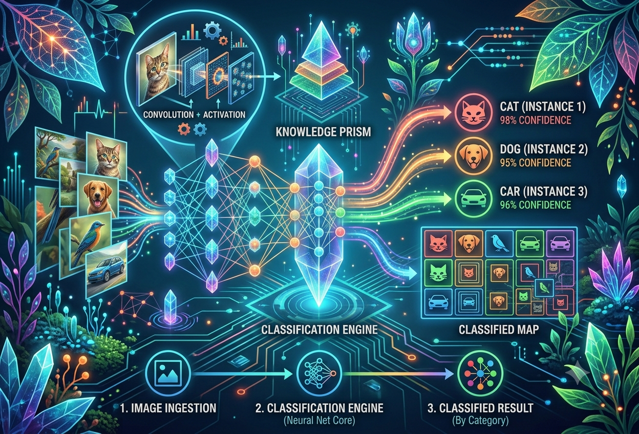
Image Classification
What Is Image Classification?
Hold up any photograph and a person can usually name what’s in it in less than a second — “that’s a dog,” “that’s a sunset,” “that’s my grandmother’s kitchen.” Image classification is the branch of artificial intelligence that teaches a computer to do that exact same trick: look at a picture and confidently announce a single label for the whole thing.
“Image classification asks a single, deceptively simple question of a photograph: given everything the system has learned, what is the one label that best describes this entire image?”— A Working Definition Used Across Computer Vision Research
Formally, image classification is a supervised machine learning task in which a model is shown thousands or millions of pictures that already carry the correct answer attached to them — a process called labeling — and the model gradually figures out the visual patterns that separate one label from another. Once trained, it can be shown a brand-new photo it has never seen before and predict which category it most likely belongs to, along with a confidence score for that guess.
Here’s a simple way to think about it: imagine you had only ever seen golden retrievers in your whole life. If someone showed you a poodle for the first time, you might hesitate, or even guess “dog, but a strange one.” An AI model trained on a narrow set of example pictures makes the very same kind of mistake — its idea of “dog” is only as wide as the photos it was allowed to study.
Think of image classification like a giant game of “Guess Which Bin.” You show the computer a picture, and it has to drop that picture into the correct labeled bin — “cat,” “bicycle,” “pizza,” “school bus.” The computer has practiced this game millions of times using example pictures with the correct bin already written on them, so by the time you show it a brand-new picture, it has gotten really, really good at guessing the right bin.
How It Differs From Other Computer Vision Tasks
People often lump “AI that looks at pictures” into one big bucket, but computer vision is actually made of several distinct jobs. Image classification is the simplest and most fundamental of them — it answers “what is this, overall?” rather than “where exactly is it?” or “which pixels belong to it?”
One label for the entire picture. “This photo contains a cat.” No location, no boundary — just a category for the whole frame.
Finds every object in the picture and draws a box around each one, with its own label. “Cat at this spot, sofa at that spot.”
Goes pixel by pixel, coloring in the exact outline of every object — far more precise, and far more computationally demanding.
Why Image Classification Matters So Much
It is easy to dismiss “a computer that names what’s in a photo” as a neat party trick. In reality, this one capability quietly sits underneath an enormous number of products and decisions that touch daily life — often without anyone noticing it is there at all.
When you unlock your phone with your face, when your photo app automatically gathers every picture of your dog into one album, when a spam filter recognises an image attached to a phishing email, when a doctor’s scanning software flags a suspicious shadow on an X-ray — image classification is the engine running quietly underneath. Unlike a single human expert who can only look at one image at a time, a trained classification model can examine thousands of images every second, every day, without ever getting tired.
From Capturing Light to Taking Action
Every real-world use of image classification follows roughly the same four-step rhythm, whether it is happening inside a phone, a hospital, or a tractor.
As classification models get folded into bigger decisions — approving an insurance claim photo, screening airport baggage, or flagging a road sign for a self-driving car — a tiny mistake no longer stays tiny. A model that is 99% accurate still gets one out of every hundred images wrong, and at the scale of millions of images a day, that “rare” mistake happens constantly. This is why accuracy alone is never the whole story; understanding where and how a model fails matters just as much.
How Computers “See” Images
A computer does not “look” at a photo the way you do. It has no eyes, no visual cortex, and no sense of beauty. What it actually receives is an enormous grid of numbers — and everything an AI model does afterward is just clever arithmetic performed on that grid.
Every digital photograph is made of tiny squares called pixels, arranged in rows and columns like a giant mosaic. A typical smartphone photo might contain over twelve million pixels. Each pixel, in turn, is usually described using three numbers — one each for how much Red, Green, and Blue light it contains, a system known as the RGB color model. Mixing different amounts of these three colors of light can reproduce almost any color the human eye can perceive.
Imagine a giant sheet of graph paper where every tiny square has been colored in by mixing just three crayons: red, green, and blue. If you use a lot of red and green crayon but no blue, that square looks yellow. A computer “sees” a photo as nothing more than a giant spreadsheet of these three crayon amounts, repeated for every single tiny square on the page.
| Pixel Property | What It Means | Typical Range |
|---|---|---|
| Red Channel | How much red light is present at that exact point in the image | 0 (none) to 255 (full) |
| Green Channel | How much green light is present at that point | 0 to 255 |
| Blue Channel | How much blue light is present at that point | 0 to 255 |
| Grayscale Value | A single brightness number used when color is not needed | 0 (black) to 255 (white) |
| Resolution | The total count of pixels — width multiplied by height | From 28×28 (tiny) to 4000×3000+ (modern cameras) |
Before any model can study a photo, it almost always needs to be resized to a fixed, smaller resolution — commonly somewhere between 224×224 and 256×256 pixels for everyday classification systems. This keeps every image the same shape and dramatically reduces how much arithmetic the computer has to perform, while usually preserving enough visual detail to still recognise the subject.
The Classification Pipeline, Step by Step
Behind every confident “that’s a cat” lies a much longer journey than most people imagine. Building a working image classifier usually moves through six distinct stages, each one capable of making or breaking the final result.
Step 1 — Collecting & Labeling Data
Everything starts with examples. Engineers gather a large pool of photographs — sometimes scraped from the web, sometimes captured specifically for the project, sometimes donated by users — and then attach the correct label to each one. This labeling work is often done by trained human annotators using specialised data-labeling platforms, since a model can only ever be as trustworthy as the labels it was taught with. Mislabeled or sloppy data quietly poisons everything that follows.
Step 2 — Preprocessing
Raw photographs arrive in every shape, size, lighting condition, and file format imaginable. Preprocessing standardises all of that chaos: images get resized to a consistent resolution, pixel values are rescaled (often from the 0–255 range down to 0–1) so the math stays stable, and inconsistent color formats are unified. Think of this step as tidying a messy desk before starting any real work.
Step 3 — Data Augmentation
Collecting millions of fresh photographs is expensive and slow, so practitioners often stretch their existing dataset further using data augmentation — automatically creating slightly altered copies of the same images so the model learns to recognise a subject under many conditions, not just one.
- Horizontal Flip: Mirrors the image left-to-right, useful since most objects look equally valid either way.
- Random Crop: Cuts out a slightly different section of the photo, teaching the model that the subject does not always sit dead-center.
- Rotation: Tilts the image a few degrees, since real cameras are rarely held perfectly level.
- Color Jitter: Nudges brightness, contrast, or saturation, simulating different lighting and camera settings.
- Random Noise: Sprinkles in tiny pixel-level static, helping the model stay steady when real-world photos are slightly grainy or blurry.
Step 4 — Splitting the Data
Before training begins, the labeled dataset is carefully divided into three separate pools so that the model is always tested on photographs it has genuinely never encountered before.
| Split | Typical Share | Purpose |
|---|---|---|
| Training Set | ~70–80% | The photos the model actually studies and learns patterns from |
| Validation Set | ~10–15% | Used to tune settings and catch problems while training is still underway |
| Test Set | ~10–15% | Locked away until the very end, used only once to measure true performance |
Imagine you are studying for a spelling test. The training set is like the practice words you study from. The validation set is like a quick mini-quiz your friend gives you to see how you’re doing. The test set is like the real spelling test on test day — you only get to take it once, and it has to contain brand-new words you have never practiced, otherwise it wouldn’t really prove you learned anything.
Types of Image Classification
Not every classification problem is the same shape. Depending on how many possible labels exist and whether an image can carry more than one label at a time, classification splits into a handful of recognisably different flavors.
Only two possible answers exist, such as “spam or not spam,” “tumor or healthy,” or “cat or not-cat.” This is the simplest version of the problem and is often where beginners start.
The model picks exactly one label out of many possible categories — for example, deciding whether a photo shows a cat, dog, horse, or rabbit, choosing only one.
A single image can rightfully carry several labels at once — a photo of a beach might simultaneously be tagged “ocean,” “sand,” “people,” and “umbrella.”
Labels are organised in nested levels, like a family tree — first deciding “animal,” then narrowing to “mammal,” then finally to “golden retriever.”
Fine-Grained vs. Coarse-Grained Classification
There is another useful way to slice this up. Coarse-grained classification deals with broadly different categories that rarely get confused with each other — telling a car apart from a banana is easy even for a fairly simple model. Fine-grained classification is far harder: distinguishing a Labrador from a Golden Retriever, or one species of butterfly from a nearly identical cousin species, requires the model to notice extremely subtle visual differences that even some humans would miss.
A medical model trying to tell “cancerous” from “healthy” tissue is doing fine-grained classification under enormous pressure — the visual differences can be genuinely tiny, and getting it wrong carries real consequences. This is exactly why medical imaging models are trained on carefully curated, expert-labeled datasets rather than casually scraped internet photos.
Classical Machine Learning Approaches
Long before deep learning became the default choice, researchers were already teaching computers to classify images — they just had to do far more of the thinking themselves. This earlier generation of methods is often called classical or traditional machine learning, and many of its ideas are still useful today, especially when data or computing power is limited.
The biggest difference between classical methods and modern deep learning lies in one phrase: handcrafted features. A classical system cannot learn directly from raw pixels — a human engineer first has to decide which mathematical descriptions of the image are worth measuring, and only those measurements get fed into the algorithm.
Extracting Features by Hand
- Color Histograms: Counts how often each color or brightness level appears anywhere in the image, useful for distinguishing scenes with very different overall color tones.
- Edge Detection: Highlights the boundaries where brightness changes sharply, since the outline of an object often carries most of its identifying shape.
- Texture Descriptors (GLCM): Measure how rough, smooth, or repetitive a surface pattern looks, helpful for telling fabric, skin, or terrain types apart.
- HOG (Histogram of Oriented Gradients): Captures the direction that edges point in across small patches of the image, historically popular for detecting human shapes.
- SIFT (Scale-Invariant Feature Transform): Finds distinctive “keypoints” in an image that stay recognisable even if the photo is rotated, resized, or taken from a slightly different angle.
Once these handcrafted numbers were extracted, they were handed off to a classical algorithm whose only job was to learn the boundary between categories using those numbers.
| Algorithm | Core Idea | Strength | Weakness |
|---|---|---|---|
| K-Nearest Neighbors (KNN) | Looks at the closest matching examples in feature-space and votes on the majority label | Simple, no real training step required | Slow to make predictions on large datasets |
| Support Vector Machine (SVM) | Draws the widest possible dividing line between categories | Performs well even with limited data | Struggles as the number of categories grows large |
| Decision Tree | Asks a sequence of yes/no questions about the features | Easy to interpret and explain | Prone to memorising noise (overfitting) |
| Random Forest | Combines many decision trees and averages their votes | More accurate and stable than a single tree | Harder to interpret than one tree alone |
| Naive Bayes | Uses probability theory, assuming features are independent of each other | Extremely fast to train | The independence assumption rarely holds perfectly for images |
K-Nearest Neighbors is like asking your five closest friends what they think a mystery food is, just by describing it. If four out of five friends say “that sounds like a mango,” you go with mango — even though none of you have actually tasted it yet. The computer does the same thing, just comparing measurements instead of descriptions.
Strengths of Classical ML
- Works reasonably well with small datasets
- Needs far less computing power to train
- Results are usually easier to explain and audit
- Faster to experiment with on a laptop
Limitations of Classical ML
- Accuracy plateaus on complex, real-world images
- Requires a human expert to design good features
- Struggles with lighting, angle, or background changes
- Mostly outperformed by deep learning since 2012
The Deep Learning Revolution: CNNs Explained
Classical methods asked humans to decide what to look for. Deep learning flipped that arrangement completely — instead of being handed handcrafted features, the model is given raw pixels and learns, entirely on its own, which patterns actually matter.
The breakthrough tool behind this shift is the Convolutional Neural Network, almost always shortened to CNN. A CNN is built from stacked layers that each transform the image a little further, starting with simple patterns like edges and gradually building up to entire object shapes by the time the information reaches the final layer.
Slides a small filter across the image, detecting a specific local pattern — like a vertical edge or a patch of a particular texture — wherever it appears.
Switches off negative signals and keeps positive ones, helping the network learn more complex, non-straight-line relationships in the data.
Shrinks the image representation down, keeping only the strongest signals from each small region and making the network faster and more tolerant of small shifts.
Combines everything the earlier layers detected into one final decision, weighing all the evidence together.
Randomly switches off some connections during training, forcing the network to avoid relying too heavily on any single shortcut.
Converts the network’s raw scores into clean probabilities that add up to 100%, one for each possible category.
Imagine sliding a tiny magnifying glass over a photo, square inch by square inch, just looking for one specific clue — say, “is there a curved line here?” Now imagine doing that thousands of times with thousands of different magnifying glasses, each looking for a different tiny clue: fur texture, pointy ears, a wet nose. The network combines all those tiny clues together, like puzzle pieces, until it’s confident enough to shout “Cat!”
Crucially, none of those “magnifying glass” filters are designed by a human. During training, the network adjusts millions of internal numbers, called weights, automatically — gradually discovering on its own which visual clues are actually useful for telling categories apart. This is what people mean when they say deep learning “learns its own features.”
Milestone Architectures: A Timeline
Image classification has a surprisingly well-documented family tree. A handful of landmark models, released over roughly three decades, each solved a specific bottleneck and pushed the entire field forward.
LeNet-5
One of the earliest practical convolutional networks, built to recognise handwritten digits on bank checks — the conceptual ancestor of every CNN that followed.
ImageNet Dataset
Stanford researchers released a massive, carefully labeled photo dataset spanning thousands of categories, finally giving deep models enough data to prove their worth.
AlexNet
Trained using GPUs for speed, AlexNet crushed the ImageNet competition with a top-5 error rate of 15.3%, against a previous best of 26.2% — instantly making deep learning the new standard.
VGGNet & GoogLeNet
VGGNet showed that stacking many small filters consistently could go deeper and score well; GoogLeNet introduced a more efficient “Inception” design that used fewer computing resources for similar accuracy.
ResNet
Introduced “skip connections” that let information bypass layers, finally allowing networks over 100 layers deep to train successfully — and reached a 3.57% top-5 error rate, beating the reported human benchmark of 5.1%.
SENet & The Transformer Paper
SENet pushed ImageNet error down to roughly 2.25%, while a separate paper in language AI quietly introduced the “Transformer” architecture that would later reshape computer vision too.
Vision Transformer (ViT)
Researchers showed that an image, chopped into patches and fed through a Transformer instead of a CNN, could match or beat convolutional networks — opening an entirely new architectural family.
Efficient & Hybrid Models
Architectures like ConvNeXt, Swin Transformer, and EfficientNet blend the strengths of CNNs and Transformers, chasing higher accuracy while using less energy and memory.
“An unequivocal turning point in the history of computer vision.”
— Yann LeCun, describing AlexNet’s 2012 ImageNet winTraining & Measuring Accuracy
Building a model is only half the job — proving that it actually works, and understanding exactly how it fails, is just as important. This section unpacks how training happens and how performance gets measured honestly.
How a Model Actually Learns
During training, the model makes a prediction, compares it against the correct label using a mathematical measurement called a loss function, and then nudges its internal weights very slightly in whichever direction reduces that loss — a process called backpropagation, repeated using an optimisation method known as gradient descent. This cycle repeats across the entire training set many times, called epochs, with the model getting a little better with every pass.
Overfitting happens when a model memorises its training examples too closely, including their quirks and noise, and then performs poorly on new photos it hasn’t seen. Underfitting happens when a model hasn’t learned enough yet and performs poorly everywhere, even on training data. The goal sits carefully in between: a model that has genuinely learned general patterns rather than memorising specific pictures.
Reading a Confusion Matrix
A confusion matrix is a simple table that lays out exactly what a model got right and wrong, broken down by category — far more informative than a single accuracy number. Here is a simplified example for a model trying to tell cats from dogs across 100 test photos:
| Predicted: Cat | Predicted: Dog | |
|---|---|---|
| Actually a Cat | 42 (correct) | 8 (missed) |
| Actually a Dog | 5 (false alarm) | 45 (correct) |
- Accuracy: The share of all predictions that were correct — here, (42+45)/100 = 87%.
- Precision: Out of everything labeled “cat,” how many really were cats — 42 / (42+5) = roughly 89%.
- Recall: Out of every real cat photo, how many did the model actually catch — 42 / (42+8) = 84%.
- F1 Score: A single balanced number that blends precision and recall together, useful when both false alarms and missed cases matter.
Imagine a metal detector at an airport. Accuracy is how often it gets the right answer overall. Recall is how good it is at catching every single dangerous item, even if it sometimes beeps at harmless belt buckles too. Precision is how often a beep actually means something dangerous, rather than a false alarm. Sometimes you care more about catching everything (high recall); sometimes you care more about not annoying everyone with false alarms (high precision).
Why does accuracy alone not tell the whole story? Imagine a dataset where 95 out of 100 photos are dogs and only 5 are cats. A lazy model that always guesses “dog” would score a misleadingly high 95% accuracy while being completely useless at recognising cats — which is exactly why a confusion matrix, precision, and recall matter so much more in practice.
Real-World Applications Across Industries
Image classification has quietly moved out of research labs and into nearly every industry that produces or relies on visual information. Here is a tour of where it is doing real, measurable work today.
Healthcare & Medical Imaging
Helps radiologists flag suspicious patterns in X-rays, MRIs, and skin photographs, acting as a tireless second opinion that highlights areas worth closer human review.
Agriculture
Identifies crop diseases, pest damage, and weeds from drone or phone photos, allowing farmers to treat exactly the affected patches instead of an entire field.
Retail & E-commerce
Powers “search by photo” shopping tools and automatically tags or sorts inventory images, making huge product catalogs searchable in seconds.
Security & Surveillance
Flags unusual objects or activity in camera feeds and supports access-control systems, though this use case carries serious privacy responsibilities.
Automotive & Transportation
Recognises traffic signs, lane markings, pedestrians, and other vehicles, forming one layer of the perception stack inside advanced driver-assistance and autonomous systems.
Manufacturing & Quality Control
Spots scratches, dents, or assembly errors on a production line far faster and more consistently than a human inspector working an eight-hour shift.
Wildlife & Conservation
Sorts through millions of motion-triggered camera-trap photos to identify species, helping researchers track endangered animal populations without endless manual review.
Satellite & Geospatial Imagery
Classifies land use, deforestation, flood extent, and urban growth from satellite photos, supporting disaster response and environmental monitoring at a planetary scale.
“The same handful of pixels-into-a-label idea quietly runs underneath farming, medicine, retail, and outer space — that breadth is exactly why image classification deserves to be understood, not just used.”
— Field Observation, Computer Vision PracticeChallenges & Trade-offs
Image classification is powerful, but it is not magic, and it is certainly not flawless. Understanding its weak points is just as important as understanding its strengths.
Strengths
- Operates at massive speed and scale, tirelessly
- Consistent — does not get bored, tired, or distracted
- Many strong pretrained models are freely available
- Improves measurably as more good data is added
Limitations
- Hungry for large amounts of accurately labeled data
- Training large models demands significant computing power and energy
- Can inherit and amplify bias hidden in training data
- Struggles badly with situations it has never seen before
Five Challenges Worth Understanding Deeply
- Data Hunger: High-performing deep models typically need thousands or millions of labeled examples per category, which is expensive and slow to collect for rare or specialised subjects.
- The Black Box Problem: Modern networks contain millions of internal numbers, making it genuinely difficult to explain in plain terms exactly why a model made a particular decision.
- Bias & Fairness: If a training dataset over-represents certain lighting conditions, skin tones, or object styles, the model’s accuracy quietly drops for everything it under-represented.
- Adversarial Vulnerability: Tiny, carefully crafted changes to an image — sometimes invisible to a human eye — can trick a model into a wildly wrong prediction with high confidence.
- Domain Shift: A model trained on bright, clean studio photos can fail badly on blurry, poorly lit, real-world phone photos that look statistically different from its training data.
Imagine someone sticks a tiny, oddly patterned sticker onto a stop sign. A human driver would still instantly recognise it as a stop sign and slow down. But certain AI models, in carefully designed experiments, have been fooled by exactly this kind of trick into thinking the sign means something completely different. This is called an “adversarial attack,” and it’s a big reason why safety-critical AI systems get tested so thoroughly before they’re trusted with real decisions.
Tools, Frameworks & Getting Started
If any of this has sparked curiosity about actually building a classifier, the good news is that the barrier to entry has never been lower. A surprising amount of professional-grade tooling is free, open-source, and well documented.
An extremely popular deep learning framework favored by researchers for its flexibility and large, active community.
A widely used framework pairing, known for being approachable for beginners while still scaling to production systems.
The standard toolkit for classical machine learning algorithms like SVMs, decision trees, and KNN, ideal for smaller datasets.
A long-standing computer vision library handling image loading, preprocessing, and classical feature extraction tasks.
A hub offering thousands of free pretrained vision models, including modern Vision Transformers, ready to fine-tune on a custom dataset.
Specialised tools for labeling images quickly and consistently at scale, an essential ingredient long before any model training begins.
Beginner-Friendly Datasets to Practice On
| Dataset | Image Size | Categories | Best For |
|---|---|---|---|
| MNIST | 28×28, grayscale | 10 (digits 0–9) | Absolute beginners, very fast to train |
| Fashion-MNIST | 28×28, grayscale | 10 (clothing items) | A slightly tougher MNIST alternative |
| CIFAR-10 | 32×32, color | 10 (animals & vehicles) | Learning CNN basics with real color images |
| Dogs vs. Cats | Variable, color | 2 | A fun, intuitive binary classification project |
| ImageNet-1K | Variable, color | 1,000 | Benchmarking serious, large-scale models |
Rather than training a network completely from scratch, most beginners get far better results, far faster, by starting with a model that has already been pretrained on a huge dataset like ImageNet, and then fine-tuning it on a smaller, specific dataset. This approach, called transfer learning, lets you stand on the shoulders of a model that has already learned to recognise edges, textures, and shapes — you only need to teach it your specific categories on top of that foundation.
The Road Ahead for Image Classification
Image classification has matured from a research curiosity into dependable, widely deployed technology. But the field is still moving quickly, and several emerging directions are reshaping what comes next.
Models trained on enormous pairs of images and their text descriptions can classify entirely new categories just from a written description, without ever being explicitly trained on that exact category.
TrendNewer models can recognise a brand-new category after seeing just a handful of examples — or sometimes none at all — rather than requiring thousands of labeled photos per class.
TrendCompact, efficient models now run directly on phones, cameras, and small sensors, classifying images instantly without sending data to a remote server — better for both speed and privacy.
TrendComputer-generated images are increasingly used to supplement real photos, helping cover rare situations that are too dangerous, expensive, or uncommon to photograph at scale.
TrendNew techniques are making it easier to visualise exactly which pixels a model focused on when making a decision, chipping away at the long-standing “black box” problem.
TrendGrowing effort is going into building training data that fairly represents different geographies, lighting conditions, and demographics, reducing the gaps that earlier datasets left behind.
TrendOpen Challenges That Remain
- Energy Footprint: Training the largest modern vision models consumes substantial electricity, raising real questions about environmental cost as models keep growing.
- Long-Tail Categories: Rare objects and species, by definition, have very few example photos, and models continue to underperform on exactly these uncommon cases.
- Robustness in the Wild: Lighting, weather, camera quality, and unexpected angles still trip up models that perform beautifully in clean, controlled test conditions.
- Privacy & Consent: As classification spreads into surveillance and identification use cases, questions about consent, data ownership, and appropriate use grow more urgent every year.
At its core, image classification is still the same simple idea it has always been: turning a grid of colored numbers into a single, useful label. What has changed dramatically is how that label gets learned — from painstaking, handcrafted rules, to deep networks that teach themselves, to models flexible enough to recognise categories they were never explicitly shown. Understanding that journey is the clearest way to understand modern computer vision itself.
Enterprise-oriented explainer covering core definitions, common techniques, and practical use cases for image classification.
A practitioner-focused walkthrough of building image classification models with machine learning, including data and tooling considerations.
A foundational overview aimed at teams getting started with classification projects and data annotation workflows.
An educational breakdown of classical and modern machine learning approaches applied to image classification problems.
A practical 2024 guide covering image classification fundamentals with an emphasis on real-world robotics and edge deployment.
A concept-level introduction explaining how image classification fits within the broader computer vision landscape.
A data-extraction-industry perspective on how image classification supports document and visual data processing workflows.
A tutorial-style article walking through classical algorithms such as SVM and KNN applied to image classification tasks.
An overview of image classification concepts with attention to dataset preparation and labeling considerations.
A comparative guide to selecting between classical and deep learning algorithms based on project constraints.
A peer-reviewed academic paper examining methods and performance considerations in image classification research.
A peer-reviewed journal article contributing technical analysis on image classification methodology.
An accessible introduction to how deep learning approaches the image classification problem, aimed at newer practitioners.
A widely used technical reference explaining image classification concepts, algorithms, and applications for learners.