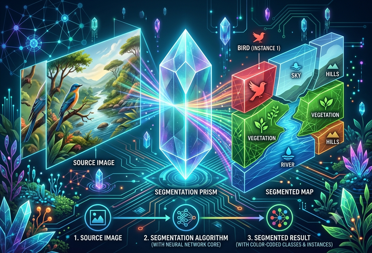
Image Segmentation
What Is Image Segmentation?
Imagine handing a child a black-and-white outline of a busy street — a car, a tree, a dog, a stretch of sky — and a box of crayons, and asking them to colour in every single region with a different colour. Image segmentation is what happens when a computer does exactly that job on a real photograph, automatically, pixel by pixel, in a fraction of a second.
Image segmentation is the process of dividing a digital photograph into separate, meaningful regions — usually one region per object or surface — by labelling every individual pixel rather than describing the picture as a single whole.— A Working Definition Used Across Computer Vision
Every photograph a computer “looks at” is really just a giant grid of numbers — one set of numbers for every tiny coloured dot, or pixel, that makes up the image. A typical photo might contain millions of these pixels. Image segmentation is the technique of sorting that enormous grid of numbers into groups, where every pixel belonging to the same object or surface gets the same label. The sky becomes one group, the road becomes another, each car becomes its own group, and so on.
This is a much harder and more useful task than simply naming what’s in a picture. A computer that can only say “this photo contains a car” knows almost nothing useful about where that car is, how big it is, or what shape it has. A computer that can shade in the exact outline of that car, pixel by pixel, can be trusted to do things like steer a vehicle around it, measure it, or remove it from the background of a video call.
Think of a join-the-dots colouring book, except instead of you tracing lines with a crayon, the computer has already figured out exactly which dots belong to the cat, which belong to the sofa, and which belong to the wall behind them — and it has filled in each one with its own colour, without ever being told in advance what a “cat” or a “sofa” looks like in that particular photo.
A Few Other Names You Might Hear
Different books, courses and engineers sometimes describe the same basic idea using slightly different words. Here are three you’ll run into often:
Because the computer is essentially running a tiny classification decision — “what category am I?” — separately for every single pixel in the image.
Unlike a model that outputs one label for a whole photo, a segmentation model outputs a prediction for every location in the image — a “dense” grid of answers rather than a single one.
The final output — a same-sized image where each pixel’s colour represents its class — is usually called a segmentation mask, since it sits over the original photo like a stencil.
Why Image Segmentation Matters
Computer vision researchers usually talk about three different “levels” of understanding a photograph, each one more detailed — and more useful — than the last. Segmentation sits at the deepest level, and that extra detail is exactly what makes so many modern technologies possible.
The first and simplest level is image classification: looking at a whole photo and attaching a single label to it, such as “cat” or “street scene.” The second level is object detection: drawing a rectangle, called a bounding box, around each object of interest and labelling it — useful, but still rough, since a rectangle around a person also includes bits of whatever is standing behind them. Image segmentation is the third and most precise level: instead of a rectangle, the computer traces the exact pixel-by-pixel outline of every object, so there’s no wasted space and no ambiguity about where one thing ends and another begins.
That extra precision is the reason segmentation quietly powers far more of daily life than most people realise. When a video-calling app blurs or replaces the background behind your face, it is running a segmentation model in real time to separate “you” from “everything behind you,” pixel by pixel, dozens of times per second. When a smartphone camera app applies a portrait blur or a quirky filter, it is doing the same thing. Self-driving cars rely on segmentation to tell the exact, pixel-accurate shape of the road, the lane markings and every pedestrian, because a rough bounding box simply isn’t precise enough when the margin for error is a few centimetres.
In medical imaging, a bounding box around a tumour might tell a doctor roughly where it is — but treatment planning, especially for radiation therapy, depends on knowing the tumour’s exact shape and volume so that healthy tissue around it is left untouched. The difference between a box and a precise pixel mask, in that context, can be the difference between a successful treatment plan and an unnecessarily damaging one.
How Machines Learn to Slice a Picture
However it’s eventually done, every segmentation method boils down to answering the same basic question for each pixel: “which of my neighbours am I most like, and which am I different from?” Computer vision researchers group the possible answers to that question into two broad strategies.
Two Basic Strategies
The similarity approach looks for pixels that share something in common — colour, brightness, texture — and groups them together into a single region, the same way you might group a basket of fruit by colour rather than by name. The discontinuity approach does the opposite: instead of looking for sameness, it hunts for sudden changes — the sharp line where a dark roof meets a bright sky — and treats those sudden jumps as the boundary between two different regions. Most real segmentation systems, whether decades-old or built only last year, lean on some mixture of these two ideas.
Imagine you’re cutting out shapes from a magazine page using scissors. One way to decide where to cut is to look for big blocks of the same colour and just cut around the whole block (that’s the similarity approach). Another way is to look for the sharp edge where one colour suddenly stops and another begins, and cut exactly along that line (that’s the discontinuity approach). Either way, you end up with neatly separated pieces.
The General Pipeline
Modern, learning-based segmentation systems follow a fairly consistent pipeline, whether they’re built around a small custom model or a giant foundation model. An input photograph is first passed through an encoder, a stack of layers that compresses the image down into a smaller grid of “features” — abstract descriptions of edges, textures and shapes rather than raw colour values. That compressed representation is then handed to a decoder, which gradually expands it back out, layer by layer, until it has rebuilt a full-sized output: a mask the same dimensions as the original photo, except now every pixel holds a class label instead of a colour.
An important engineering detail hides inside that “compress, then expand” idea: the more aggressively an encoder compresses an image, the more precise positional information it tends to throw away — exactly the kind of information a segmentation task can’t afford to lose. That’s why many segmentation networks deliberately avoid heavy compression techniques (like aggressive pooling) in favour of gentler downsampling that keeps better track of where things were in the original photo, a theme we’ll return to in the deep learning models below.
One simple mental model: imagine sliding a piece of black construction paper, with a hole cut to the exact shape of an object, over a photograph. Everything inside the hole is “kept,” and everything else is hidden. A segmentation mask works the same way, except a single image usually contains several of these “cut-outs” stacked together — one per object or surface — rather than just one.
Semantic, Instance & Panoptic Segmentation
Not every segmentation task needs the same level of detail. Computer vision researchers split the field into three flavours, each one answering a slightly more demanding question than the last.
“Things” and “Stuff”
Before getting into the three types, it helps to know one piece of vocabulary researchers use constantly: the difference between things and stuff. “Things” are countable objects with a clear, consistent shape — a car, a person, a dog. You can point at one and say “there’s another one.” “Stuff” refers to regions that don’t really come in countable units — sky, grass, water, road. You wouldn’t usually say “there are three skies in this photo.” This distinction matters because the three types of segmentation below treat things and stuff quite differently.
Labels every pixel with a category — “road,” “car,” “sky” — but never distinguishes between two objects of the same category. Three parked cars become one big “car” region.
Tells individual objects of the same category apart — “car 1,” “car 2,” “car 3” — but generally ignores background “stuff” like sky or road entirely.
Combines both: every pixel gets a category label, and every individual “thing” also gets its own instance number. Nothing in the photo is left unlabelled.
| Type | What It Tracks | Typically Used For |
|---|---|---|
| Semantic | One class label per pixel; identical objects merge into one region | Road-scene understanding, background removal, scene parsing |
| Instance | A unique boundary for every individual object; ignores background “stuff” | Counting objects, tracking, AR/VR object isolation |
| Panoptic | A class label and an instance number for every pixel | Autonomous driving, robotics, full scene understanding |
Picture a photo of two pet cats sitting on a rug. A semantic-segmentation computer would colour both cats the same shade of orange and just call them “cat.” An instance-segmentation computer would notice they’re two separate cats and colour one orange and the other purple, calling them “cat 1” and “cat 2” — but it might not bother colouring the rug at all. A panoptic-segmentation computer does both jobs at once: two different cat colours, plus a colour for the rug too, so absolutely nothing in the photo is left blank.
Classic Segmentation Techniques
Long before neural networks were practical, engineers were already segmenting images using clever mathematics applied directly to pixel brightness and colour. These “classic” techniques are decades old, but they remain fast, cheap to run, and perfectly adequate for plenty of simpler tasks today — which is why they’re still taught first.
| Technique | Core Idea | Good For |
|---|---|---|
| Thresholding | Pick a brightness “cutoff” value; everything above it is foreground, everything below is background | Document scanning, high-contrast images |
| Edge Detection | Hunt for sudden jumps in brightness or colour and mark them as object boundaries | Objects with clean, well-defined outlines |
| Region-Based | Start from a “seed” pixel and grow outward, absorbing neighbours that look similar | Medical scans, noisy or textured images |
| Clustering | Treat every pixel’s colour as a data point and group similar points together mathematically | Colour-based simplification, quick previews |
| Watershed | Treat brightness as elevation on a map and trace where the “valleys” naturally separate | Touching or overlapping round objects, e.g. blood cells |
Thresholding: Drawing a Line in the Sand
The simplest possible segmentation method is thresholding: pick one brightness value, and sort every pixel into “above” or “below” it. Global thresholding uses one fixed cutoff for the whole image, which works nicely when lighting is even throughout. Adaptive thresholding instead calculates a separate cutoff for each small region of the photo, which copes far better with shadows or uneven lighting. A popular automatic way of choosing that cutoff, called Otsu’s method, mathematically finds the threshold that best separates an image’s two main brightness groups.
Edge Detection: Following the Outline
Edge-based methods look for places where brightness changes sharply from one pixel to the next, since that’s usually where one object ends and another begins. The best-known edge detectors — Sobel, Canny and Laplacian — each use a slightly different mathematical filter to measure that change, with the Canny detector generally producing the cleanest, most continuous outlines at the cost of being slower to compute.
Region-Based and Clustering Methods
Region-growing techniques start from one or more “seed” pixels and keep absorbing neighbouring pixels as long as they stay similar enough, like a drop of ink slowly spreading through similarly-coloured fabric. A related family, split-and-merge, works in the opposite direction — starting with the whole image as one region and recursively splitting it into quarters wherever the pixels inside are too different from each other. Clustering algorithms such as k-means take a different approach entirely: every pixel’s colour is treated as a point in space, and the algorithm repeatedly groups nearby points together until it settles on a fixed number of clusters, each becoming its own segment.
Treats the image as a tiny mountain range, where brightness becomes elevation. Imagine rain falling and pooling in the valleys — wherever two pools are about to merge, the algorithm builds a “dam,” and those dams become the segment boundaries. It’s especially good at separating touching, similarly-shaped objects, such as blood cells under a microscope.
Represents the whole image as a network, with every pixel connected to its neighbours by a “similarity” score. The algorithm then mathematically cuts that network into pieces wherever the connections are weakest, which tends to fall exactly along true object boundaries.
These methods are fast, lightweight, and require no training data at all — but they generally only understand colour, brightness and texture. They have no concept of what a “car” or a “dog” actually is, so they can be thrown off badly by shadows, reflections, or two differently-coloured parts of the very same object. That gap in understanding is exactly what deep learning was built to close.
Deep Learning Models
Starting in the mid-2010s, researchers worked out how to train neural networks to perform segmentation end-to-end — learning directly from labelled examples what a “car” or a “road” looks like, instead of relying on hand-written colour-and-brightness rules. The improvement in accuracy was so large that deep learning quickly became the default approach for anything beyond the simplest images.
The Encoder-Decoder Shape
Almost every modern segmentation network is built around the encoder-decoder idea introduced in Section 03: compress the image down, then expand it back out into a full-sized mask. The diagram below shows why these networks are so often drawn — and nicknamed — in the shape of the letter “U.”
That dashed “skip connection” line solves a real problem: compressing an image all the way down to a bottleneck necessarily throws away fine spatial detail — exactly where a thin object boundary sat, for instance. Skip connections let the decoder borrow that lost detail directly from the matching encoder layer, stitching it back in as the image is rebuilt. This single idea, introduced by the U-Net architecture, is one of the most widely copied tricks in all of modern computer vision.
The first network proved a neural network could be trained end-to-end for segmentation, by swapping a classifier’s fixed-size final layers for convolutions that work on any image size.
2015Built for biomedical images with very little training data available, its skip connections preserve fine detail — making it a long-standing favourite for medical scans.
MedicalRemembers exactly which pixel each “important” feature came from during compression, so it can put that feature back in precisely the right spot during decoding — handy for street-scene understanding.
ScenesUses “atrous” (deliberately gappy) convolutions to see a wider area of the image without shrinking it as aggressively, capturing context at multiple scales efficiently.
v1 – v3+A two-stage instance-segmentation model: first it proposes likely object regions, then it refines each one into a precise mask, a class, and a bounding box.
InstanceBorrows the “attention” mechanism from language models, letting every patch of the image directly weigh how relevant every other patch is — useful for understanding distant relationships in a scene.
AttentionTwo Ways to Find Individual Objects
For instance segmentation specifically, models tend to follow one of two broad strategies. Two-stage models, like Mask R-CNN, first propose candidate regions and then carefully refine each one — trading speed for accuracy. One-shot models, in the style of YOLO, perform detection, classification and mask generation all in a single pass through the network, trading a little accuracy for the speed needed to run in real time, such as on a moving vehicle’s camera feed.
Fully Convolutional Networks & U-Net
The first end-to-end trainable segmentation networks arrive within months of each other, one general-purpose and one tailored for medical images.
SegNet, DeepLab v1 & Mask R-CNN
Encoder-decoder designs mature, atrous convolutions arrive, and instance segmentation becomes practical at scale.
DeepLab v3+ & Vision Transformers
Encoder-decoder refinements continue, while attention-based transformer architectures begin matching or beating convolutional networks on segmentation benchmarks.
Segment Anything Model (SAM)
Meta releases a single foundation model trained on over a billion masks, able to segment objects it has never specifically been trained on, simply from a point or box prompt.
You can think of older segmentation networks as students who had to study one very specific subject really hard — say, only “medical scans” or only “street photos.” SAM is more like a student who has read so many different books on so many different topics that you can now just point at almost anything in a brand-new photo and ask “what’s the outline of this?” — and it can usually give you a good answer, even if it has never seen that exact object before.
Where Image Segmentation Lives
Once you know what to look for, image segmentation turns up almost everywhere a camera and a computer meet. Here’s a tour of the industries leaning on it most heavily today.
Healthcare & Medical Imaging
Outlining tumours, organs and tissue boundaries in MRI, CT and X-ray scans for diagnosis, treatment planning, and tracking how a disease changes over time.
Autonomous Vehicles & Robotics
Identifying drivable road surface, lane markings, pedestrians and obstacles with pixel-level precision, where a rough bounding box simply isn’t safe enough.
Agriculture
Telling individual crops, weeds and diseased leaves apart from drone or satellite imagery to guide targeted spraying, irrigation and yield estimates.
Satellite & Environmental Monitoring
Mapping land cover, tracking deforestation, monitoring urban growth, and even spotting illegal mining sites from space by segmenting terrain types over time.
Retail & Fashion
Isolating individual clothing items for virtual try-on experiences, automated cataloguing, and visual search (“find this exact jacket”).
Security, Surveillance & Privacy
Identifying people and vehicles in video footage for monitoring — and, just as importantly, precisely masking faces and licence plates to protect privacy during video redaction.
Manufacturing & Quality Control
Spotting cracks, dents and surface defects on a production line by segmenting them away from a flawless background, far faster than a human inspector.
Social Media, AR & Photography
Powering camera filters, virtual backgrounds, and portrait-mode blur effects by separating a person or object from everything behind them in real time.
“Once an image has been segmented, a computer is no longer looking at a flat picture — it’s looking at a small map of distinct, individually addressable objects.”
— A Common Way Computer Vision Engineers Explain the PayoffPros & Cons of Image Segmentation
Like any powerful tool, image segmentation comes with real trade-offs. Knowing both sides helps in deciding when it’s the right technique to reach for — and when a simpler one, like classification or detection, will do the job just fine.
Advantages
- Pixel-level precision enables tasks where a rough estimate simply isn’t acceptable, such as surgical planning
- Pre-segmenting an image can speed up later processing steps, since a detector only has to examine the relevant region
- Foundation models like SAM now generalise to brand-new objects with little or no extra training
- Works across an unusually wide range of domains — medical scans, satellite photos, street scenes and product photography alike
- One-shot models can run in real time, even on the modest hardware inside a phone or a car
Drawbacks
- Deep learning approaches are computationally demanding, often needing GPUs for both training and fast inference
- Struggles with cluttered backgrounds, heavy occlusion, and objects that overlap closely
- Training data is expensive: every pixel in every training image must be carefully, manually labelled
- Performance often drops sharply on rare or unusual object categories the model has barely seen before
- Integrating a segmentation model into an existing software pipeline can be a non-trivial engineering task on its own
How We Score a Segmentation
If a computer colours in a photo, how do we know whether it did a good job? Researchers compare the computer’s predicted mask against a carefully hand-labelled “ground truth” mask, and reduce that comparison to a single, easy-to-track number.
Intersection over Union (IoU)
The most widely used metric, also called the Jaccard index, works in three simple steps: find the area where the prediction and the ground truth overlap (the intersection), find the total area covered by either one of them (the union), and divide the first number by the second. A perfect prediction scores exactly 1; a complete miss scores 0.
Dice Coefficient
Closely related to IoU, the Dice coefficient also rewards overlap between prediction and ground truth, but weighs the intersection slightly more heavily — which is why it’s often the preferred metric in medical imaging, where small structures matter a great deal. It also ranges from 0 to 1, with 1 meaning a perfect match.
Pixel Accuracy, Precision & Recall
Pixel accuracy simply asks what percentage of all pixels were labelled correctly — easy to understand, but easy to fool: a model that lazily labels an entire photo “background” can still score deceptively well if background pixels happen to dominate the image. Precision and recall dig deeper, separately measuring how often the model’s positive predictions were correct, and how many of the true positive pixels it managed to actually find.
| Metric | What It Measures | Watch Out For |
|---|---|---|
| IoU / Jaccard | Overlap area ÷ combined area, 0 to 1 | The standard, most widely reported choice |
| Dice Coefficient | A closely related overlap score that weighs intersection more heavily | Popular for small or thin structures, e.g. tumours |
| Pixel Accuracy | Percentage of all pixels labelled correctly | Misleading when one class dominates the image |
| Precision & Recall | Correctness of positive predictions vs. how many true positives were found | Useful together; neither tells the full story alone |
Imagine you traced around a leaf with your own crayon, and your friend also traced around the very same leaf with their crayon, without seeing yours. IoU is basically asking: “how much of the area inside either of our two crayon lines is actually shared by both of us?” If your outlines match almost perfectly, that shared area is huge — a high score. If your outlines barely overlap, the shared area is tiny — a low score.
The Datasets That Teach the Machines
A deep learning model is only as good as the examples it learns from. Before it can segment a brand-new photo well, it first has to study thousands — sometimes millions — of photos that humans have already painstakingly labelled, pixel by pixel, by hand.
Over 330,000 everyday photos labelled across 80 “thing” categories and 91 “stuff” categories — the most widely used general-purpose benchmark in the field.
GeneralStreet scenes captured across 50 different cities, finely annotated for the specific needs of autonomous-driving research.
DrivingOver 20,000 scene-centric images spanning roughly 150 categories, built by MIT for general scene-parsing research.
ScenesOne of the original computer-vision benchmark datasets, with 21 object categories and carefully split training, validation and test sets.
LegacyHours of real driving footage recorded around Karlsruhe, Germany, widely used for autonomous-driving and robotics research.
DrivingMeta’s enormous dataset built specifically to train SAM — roughly 11 million images carrying over 1 billion individual segmentation masks.
FoundationBuilding a dataset like these is far more laborious than it might sound. Every single pixel in every single training image has to be assigned to the correct category by a human annotator, then checked for consistency — which is exactly why these “ground truth” datasets, once created, get reused as shared benchmarks across the entire research community rather than rebuilt from scratch for every new project.
A model can only ever be judged against the quality of the labels it’s compared to. If the humans who built a dataset disagreed about exactly where an object’s edge was — which happens more often than you’d expect — that uncertainty quietly limits how “accurate” any model trained on it can ever be measured to be.
Challenges & Limitations
Despite five decades of progress, image segmentation is still not a fully solved problem. Several genuine, stubborn difficulties keep researchers busy.
- Defining “meaningful” in the first place: Two careful human annotators don’t always agree on exactly where one object ends and another begins, which makes segmentation what researchers call an “ill-posed” problem — there isn’t always one single correct answer to aim for.
- Cluttered backgrounds & low contrast: When an object’s colour and texture barely differ from its surroundings, even the best models can struggle to trace a clean boundary.
- Overlapping & occluded objects: Two objects of the same type that overlap, or an object partly hidden behind another, are notoriously hard to separate cleanly.
- Computational cost: Training and running large segmentation models, especially at high resolution or in real time, demands serious GPU power — a real barrier for smaller teams or on-device applications.
- The long-tail problem: Rare object types that appear only a handful of times in a training set are exactly the ones a model is most likely to get wrong, since it simply hasn’t seen enough examples to learn from.
- Lighting & appearance variation: The same object can look dramatically different under different lighting, weather, or camera angles, and a model trained mostly on one set of conditions can fail badly on another.
- Integration with real software: Plugging a research-grade model into a production pipeline, with all its existing data formats and performance requirements, is its own substantial engineering challenge.
Because deep learning models learn entirely from their training data, a dataset that under-represents certain conditions, regions or object types will produce a model that performs noticeably worse on exactly those cases — a limitation worth remembering any time a segmentation system is deployed somewhere far removed from the conditions it was trained on.
The Road Ahead
Image segmentation has travelled a long way — from hand-picked brightness thresholds in the 1970s to a single model that can outline almost anything you point at today. Several clear trends point to where it heads next.
Models like SAM are pushing the field away from “train one model per task” and towards general-purpose segmenters that work on objects they’ve never specifically seen, guided only by a point, a box, or even a text description.
GeneralisationResearchers are blending fast classic techniques like thresholding and clustering with deep learning, using each to initialise or refine the other for better speed and accuracy together.
HybridLighter, faster architectures are being designed to run segmentation directly on phones, drones and embedded devices, rather than relying on a distant, powerful server.
SpeedCombining segmentation with language understanding lets a person simply describe what they want isolated — “the red car,” “the smaller dog” — instead of clicking precise points.
LanguageResearchers are developing measures that go beyond simple overlap, such as boundary-specific scores, to better capture how clean and precise an object’s traced edge actually is.
MetricsExtending segmentation across time (consistently tracking an object’s mask through every frame of a video) and into three dimensions (for robotics and augmented reality) remains an active frontier.
Extensions“Every leap in image segmentation has been a leap towards machines understanding not just what is in a photograph, but exactly where it is, down to a single pixel.”
— A Common Framing in Computer Vision Research, 2026Image segmentation turns the simple question “what’s in this picture?” into the far more useful question “exactly where, down to the pixel, is everything in this picture — and how is each piece different from the next?” That single shift in precision is what allows a video call to swap your background, a car to know exactly where the road ends, and a doctor to measure a tumour to the millimetre — all from the same basic idea of colouring in a photo, one pixel at a time.
Overview of segmentation types, classic techniques, deep learning models, evaluation metrics and a classification-vs-detection-vs-segmentation comparison table.
In-depth explainer covering “things vs. stuff,” semantic/instance/panoptic segmentation, traditional techniques, deep learning models and training datasets.
Detailed guide covering segmentation types, edge/region/clustering techniques, deep learning architectures including SAM, and evaluation with IoU.
Best-practice guide with comparison tables for segmentation types and techniques, deep learning and foundation models, metrics, and benchmark datasets.
Practical overview of segmentation types, applications in data extraction, common tools and libraries, and real-world implementation challenges.
Practitioner write-up walking through segmentation concepts, techniques and implementation considerations in greater technical depth.
Technical deep dive into thresholding (including Otsu and optimal thresholding mathematics), edge-based, region-based and clustering-based segmentation.
Overview of segmentation techniques, applications across industries, and a survey of widely used image segmentation datasets.
François Chollet’s textbook chapter covering the encoder-decoder approach, training a segmentation model from scratch, IoU evaluation, and using Meta’s Segment Anything Model.
Tutorial-style overview of segmentation concepts and common techniques aimed at machine learning learners.
Explains semantic vs. instance vs. panoptic segmentation, the classification-localisation-segmentation labelling process, and everyday use cases like social media filters and Tesla’s self-driving cameras.
Explainer on the deep learning approach to segmentation, covering CNNs, RNNs and the comparative benefits over traditional techniques.
ML-basics explainer covering “things vs. stuff,” segmentation types, traditional and deep learning techniques, and real project examples in satellite-based environmental monitoring.
Covers the similarity vs. discontinuity approaches and applications in video surveillance, healthcare and privacy-focused video redaction.
Peer-reviewed academic review covering classic, co-segmentation and deep-learning-based segmentation methods, including encoder-decoder design, skip connections, dilated convolution and attention mechanisms.
Tutorial-style introduction to segmentation concepts and common technique categories for learners new to computer vision.