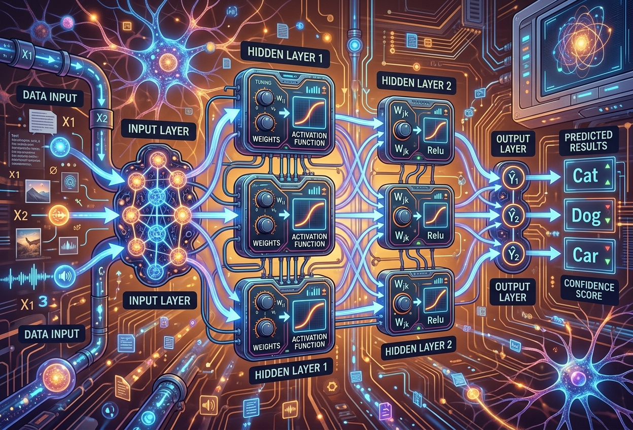
Forward Propagation
in AI
What Is Forward Propagation?
Imagine you are guessing the flavour of a mystery ice cream just by looking at its colour. You take in the information, think about it step by step, and eventually announce your best guess. That is exactly what forward propagation does inside a neural network.
Forward propagation is the step-by-step journey that data takes through a neural network — from the moment it enters as raw numbers, all the way to the moment it exits as a prediction or decision.— Core Concept · Deep Learning Fundamentals
A neural network is a computer system loosely modelled after the human brain. It is made up of many small mathematical units called neurons, organised in layers. When you feed data into the network — say, a photo of a cat — that data does not jump instantly to an answer. Instead, it travels through each layer one by one, getting transformed at every step. This whole forward journey is what computer scientists call forward propagation.
Think of it like passing a message down a very long line of people at a party. The first person hears the original message, whispers a slightly changed version to the next person, and so on down the line until the last person announces the final result. Each person represents one layer of the neural network. Each whisper represents a mathematical calculation. And the final announcement is the network’s prediction.
Picture a row of toy robots. You whisper a number to the first robot. It does a small calculation and whispers a new number to the second robot. That robot does another calculation and passes it along. Eventually, the last robot shouts out an answer. That answer is the AI’s “guess.” The entire chain of whispering is forward propagation!
Why Does Forward Propagation Matter?
Forward propagation is the very act of a neural network making a prediction. Without it, the network simply cannot do anything at all. Every time you ask an AI to identify a face in a photo, translate a sentence, suggest a song, or tell you whether an email is spam — forward propagation is running behind the scenes.
It is also the foundation for learning. Before a network can improve itself (through a separate process called backpropagation), it first has to make a prediction. That prediction comes from forward propagation. The error in that prediction is then used to teach the network. So forward propagation is not just one step — it is the heartbeat of the entire learning cycle.
- Every AI prediction starts here. Whether it is a chatbot replying to you or a self-driving car deciding to brake, forward propagation is the first computation that happens.
- It defines the network’s current “knowledge.” The weights and biases used during forward propagation encode everything the network has learned so far.
- It is needed during both training and deployment. When a network is learning, forward propagation runs before every weight update. When deployed, it runs on every new piece of data.
- Efficiency here matters enormously. In large language models serving millions of users, even tiny improvements in forward-pass speed translate to huge savings in computing cost and energy.
Anatomy of a Neural Network
Before we can trace how data moves through a network, we need to understand what a network is built from. Think of it as learning the names of the rooms in a house before taking a tour.
FIG 01 — A fully connected feedforward neural network with 3 input neurons, two hidden layers of 3 neurons each, and 2 output neurons. Every connection carries a learned weight.
The Three Types of Layers
Every neural network is organised into layers. Each layer is a group of neurons that all receive information from the previous layer, process it, and pass their results forward.
The front door of the network. Raw data enters here. If you are feeding in a 28×28-pixel image, the input layer has 784 neurons — one per pixel value. No calculation happens here; neurons simply hold the incoming numbers.
The real thinkers. One or more hidden layers sit between the input and output. This is where the network extracts patterns, finds features, and builds understanding. “Hidden” simply means we do not see their output directly — it is internal to the network.
Key LayerThe final verdict. This layer produces the network’s answer. For a cat-vs-dog classifier it might have two neurons. For a language model it might have thousands — one per word in the vocabulary.
The word “deep” in deep learning refers to the depth of a network — the number of hidden layers it contains. A shallow network has one hidden layer. A deep network might have hundreds. More depth generally means more complex and abstract patterns can be learned, but also requires more data, more computation, and more careful design.
Inside a Single Neuron
A neuron is the smallest unit of computation in a neural network. Understanding what one neuron does is the key to understanding what thousands of them do together.
Think of a neuron as a tiny decision-maker. It receives several signals from neurons in the previous layer, weighs how important each signal is, adds everything up, makes a small adjustment, and then decides whether to pass a strong signal, a weak signal, or no signal at all to the next layer.
FIG 02 — Anatomy of a single artificial neuron. Three inputs arrive with associated weights. The neuron computes a weighted sum, adds a bias, then passes the result through an activation function to produce its output.
The Four Things Every Neuron Does
Weights — The Knobs of Intelligence
Every connection between two neurons has a weight — a number expressing how important one neuron’s signal is to the next. A high positive weight says “pay close attention to this signal.” A negative weight says “this signal actually argues the other way.” A weight close to zero means “mostly ignore this.”
When we say a neural network “learns,” what we really mean is that it gradually adjusts these weights until the predictions become accurate. But adjusting happens during training, through backpropagation. During forward propagation, the weights are fixed — the network simply uses whatever values they currently hold.
Bias — The Nudge
Every neuron also has a bias — a small extra number added to the weighted sum before the activation function. Think of it as a thumb on the scale. The bias allows a neuron to shift its output up or down independently of the inputs. Without bias, every neuron receiving zero input would always output exactly zero, which would cripple the network’s ability to learn many patterns.
Imagine you are judging a cooking competition. Each dish has three qualities: taste, presentation, and aroma. You might care more about taste than aroma — so taste gets a higher weight. The bias is like your mood that day: even a zero-score dish might get a half mark just because you are in a good mood. Together, your weighted judgement plus your mood-nudge equals your score — which you then push through your personal “is this worth recommending?” filter (the activation function).
How Forward Propagation Works
Now that we know the building blocks, let us trace a piece of data as it travels through an entire neural network from start to finish. We will use a relatable example: teaching an AI to recognise whether a fruit is a mango or an apple.
Our tiny network has two inputs (sweetness and colour intensity, measured as numbers from 0 to 1), one hidden layer with three neurons, and one output neuron that produces a number between 0 and 1 — where values closer to 1 mean “mango” and values closer to 0 mean “apple.”
FIG 03 — A complete forward propagation pass through our fruit classifier. Inputs flow through weighted sums, activation functions, and produce a final prediction with a confidence score.
Step-by-Step Walkthrough
- The data enters the input layer. Our two fruit measurements — sweetness (0.9) and colour intensity (0.7) — are placed into the two input neurons. No calculations yet; the neurons simply hold these values.
- Each hidden neuron computes a weighted sum. Every neuron in the hidden layer receives both inputs (0.9 and 0.7), multiplies each by its corresponding weight, adds up the products, and then adds its bias term. This single number is called the pre-activation value, usually written as z.
- The activation function fires. Each pre-activation value z is passed through an activation function (more on this in Section 6), which decides how strongly the neuron should respond. The result — the activation — is what gets passed to the next layer.
- The process repeats through every layer. The activations from the hidden layer become the inputs to the output layer, which performs the same weighted-sum-plus-activation calculation one more time.
- The output layer produces the prediction. The final output neuron produces a number: 0.87. Since values above 0.5 mean “mango,” the network confidently classifies this fruit as a mango. Forward propagation is complete.
The Mathematics of Forward Propagation
Do not be scared by the maths here. Each equation is simply a precise way of writing down what we already described in words. We will go through each piece slowly.
The Core Equation for One Neuron
Every neuron in every layer does the same basic calculation. If a neuron receives inputs x₁, x₂, x₃ with weights w₁, w₂, w₃ and has a bias b, it first computes:
— multiply each input by its weight, sum them all, add bias
Then it applies an activation function f to get the neuron’s output:
— squash z through a function that adds non-linearity
Writing It as a Matrix Equation
In practice, an entire layer has many neurons and receives many inputs simultaneously. Writing one equation per neuron would be impossibly tedious. So we use matrices to express the calculations for a whole layer at once. For layer number l:
A[l] = f ( Z[l] )
W[l] = weight matrix of layer l (one row per neuron, one column per input)
A[l−1] = output (activations) from the previous layer
b[l] = bias vector for layer l
f = activation function applied element-wise
A[l] = the output of this layer, which feeds into the next
This pair of equations is repeated for every layer in the network, with the output of layer l becoming the input to layer l+1. The very first input A[0] is just the original data. The very last output A[L] is the network’s prediction.
Imagine you have three friends who each tell you a rumour. You trust Friend 1 a lot (weight = 0.8), you sort of trust Friend 2 (weight = 0.5), and you barely trust Friend 3 (weight = 0.1). You multiply how much each friend says by how much you trust them, add it all up, add your own gut feeling (bias), and then decide how strongly you believe the rumour. That decision IS the formula above — just written in number language!
A Worked Numerical Example
Let us trace real numbers through one layer. Suppose a hidden neuron receives two inputs: x₁ = 0.6 and x₂ = 0.4. Its weights are w₁ = 0.9 and w₂ = −0.5, and its bias is b = 0.2.
z = 0.54 − 0.20 + 0.20
z = 0.54
Applying ReLU activation: f(z) = max(0, z) a = ReLU(0.54) = max(0, 0.54) = 0.54
— ReLU keeps positive numbers unchanged and replaces negatives with 0
The neuron outputs 0.54. This value now travels forward to every neuron in the next layer, where the same process repeats.
Activation Functions
Without activation functions, a neural network — no matter how many layers it has — would behave exactly like a single linear equation. It would never be able to learn curves, waves, spirals, or any of the complex patterns that make AI genuinely useful.
Activation functions are the mechanism that introduce non-linearity into the network. They determine whether a neuron’s signal should be passed on strongly, weakly, or not at all. Think of them as tiny gates or switches inside each neuron.
FIG 04 — Three of the most commonly used activation functions. ReLU dominates hidden layers of modern networks. Sigmoid and Tanh serve specialised roles in output layers and recurrent architectures.
| Activation | Formula | Output Range | Best Used For | Key Weakness |
|---|---|---|---|---|
| ReLU | max(0, z) | [0, ∞) | Hidden layers in CNNs & feedforward nets | Dying ReLU (dead neurons) |
| Leaky ReLU | max(0.01z, z) | (−∞, ∞) | Fixing dying ReLU in deep nets | Slope is a hyperparameter to tune |
| Sigmoid | 1 / (1 + e⁻ᶻ) | (0, 1) | Binary classification output layers | Vanishing gradients in deep nets |
| Tanh | (eᶻ − e⁻ᶻ) / (eᶻ + e⁻ᶻ) | (−1, 1) | Recurrent networks (RNNs, LSTMs) | Still suffers from vanishing gradients |
| Softmax | eᶻᵢ / Σeᶻⱼ | (0, 1) summing to 1 | Multi-class classification output | Expensive for large vocabularies |
| GELU | z × Φ(z) | (≈−0.17, ∞) | Transformers (BERT, GPT, etc.) | More expensive to compute than ReLU |
Without activation functions, stacking a hundred layers is mathematically identical to having just one. It is the non-linearity that gives neural networks their almost magical ability to approximate any function imaginable.
— Core Principle · Universal Approximation TheoryForward Propagation vs. Backpropagation
Forward propagation and backpropagation are the two-stroke engine of neural network learning. One makes a guess. The other corrects the mistake. Together, they repeat thousands or millions of times until the network becomes accurate.
FIG 05 — The training cycle. Forward propagation generates a prediction and a loss value. Backpropagation uses that loss to compute gradients and update every weight in the network.
Direction: input → output (left to right). Purpose: generate a prediction. When: both during training and deployment. Updates weights? No — weights are frozen during the forward pass; it is used to apply what has been learned.
InferenceDirection: output → input (right to left). Purpose: calculate how to improve the weights. When: only during training — never during deployment. Updates weights? Yes — it computes gradients and adjusts every weight in the network.
TrainingForward propagation is like throwing a dart at a board — you make your best effort and see where it lands. Backpropagation is like looking at where you missed, figuring out how to adjust your arm angle and throw strength, and correcting your aim for the next throw. After hundreds of throws, you get very good at hitting the bullseye!
Where Forward Propagation Powers AI
Every time a neural network produces any output whatsoever — a translated sentence, a medical diagnosis, a song recommendation — forward propagation has just run. It is the universal mechanism behind all neural-network-based AI in the world today.
Healthcare & Medicine
Medical imaging systems use forward propagation to scan X-rays, MRI scans, and retinal photographs, flagging abnormalities like tumours, diabetic retinopathy, or fractures. Each pixel travels through hundreds of layers, and the final output is a probability that something unusual is present — often rivalling experienced radiologists.
Self-Driving Vehicles
Cameras, LiDAR sensors, and radar generate enormous streams of data. Dozens of forward passes run every second — identifying pedestrians, reading traffic signs, tracking moving objects, and predicting trajectories — so the vehicle can make safe navigation decisions in real time.
Natural Language Processing
Large language models behind chat assistants, translation services, and search engines perform forward propagation for every single token they process. When you ask a question and receive a reply, each word in that reply was generated by running a forward pass through billions of parameters.
Recommendation Systems
Streaming platforms use neural networks to understand your taste from what you have listened to, watched, or read. Forward propagation maps your preferences into a mathematical space and finds content closest to that point — producing recommendations personalised just for you.
Cybersecurity
Security systems run forward propagation on network traffic, email content, and user behaviour signatures to detect anomalies in real time. Because forward propagation can run on vast amounts of data at speed, it can flag threats milliseconds after they appear — far faster than any human analyst.
Agriculture & Climate
Satellite imagery and drone footage feed neural networks that assess crop health, predict yields, detect pest infestations, and model climate patterns. Forward propagation processes thousands of square kilometres of imagery to produce actionable recommendations for farmers and environmental planners.
Strengths & Limitations
Forward propagation is a beautifully simple idea executed with remarkable computational efficiency. But like every engineering approach, it carries real trade-offs worth understanding — especially as networks grow larger and are deployed in higher-stakes environments.
✓ Strengths
- Computationally efficient. A forward pass through even a large network completes in milliseconds on modern GPUs, enabling real-time AI applications.
- Parallelisable. Layer computations expressed as matrix multiplications run exceptionally well on GPUs and TPUs.
- Conceptually simple. Data flowing forward through layers of transformations is intuitive and easy to reason about — making debugging more tractable.
- Scales to enormous networks. The same operations that work for a 3-layer network also work — just with larger matrices — for networks with hundreds of billions of parameters.
- Universal applicability. Works for image, text, audio, tabular, graph, and virtually any structured input — making it the backbone of nearly all modern AI.
- Hardware optimised. Modern chips (NVIDIA H100, Google TPU, Apple Neural Engine) are purpose-built to accelerate the matrix multiplications at the heart of forward propagation.
✗ Limitations
- No internal memory between predictions. A single forward pass is stateless — recurrent or attention architectures are needed for sequence memory.
- Depends entirely on good weights. If weights are bad (poorly initialised or undertrained), forward propagation produces terrible predictions; quality mirrors training quality.
- Black-box outputs. It can be hard to explain why a particular forward pass produced a particular output — a real concern in healthcare or criminal justice.
- Vanishing/exploding values. In very deep networks, pre-activation values can shrink to near-zero or grow uncontrollably, destabilising training.
- Energy intensive at scale. Running forward propagation on billions of requests per day consumes substantial energy — raising environmental concerns.
- Sensitive to distribution shift. If real-world data looks different from training data, forward propagation will give confidently wrong outputs — a phenomenon known as distribution shift.
A Brief History of Forward Propagation
The idea of information flowing forward through connected units has roots stretching back to the very beginning of computing. Understanding this history helps explain why forward propagation looks the way it does today.
McCulloch & Pitts — The First Artificial Neuron
Warren McCulloch and Walter Pitts published a landmark paper proposing a simplified mathematical model of a biological neuron. Their model accepted binary inputs, multiplied them by weights, and produced a binary output — a primitive but recognisable ancestor of modern forward propagation.
Rosenblatt’s Perceptron — Learning from Data
Frank Rosenblatt developed the Perceptron, the first learning algorithm for a single-layer network. It could adjust its weights based on errors — a rudimentary training loop that, for the first time, made the forward computation useful beyond pure theory.
Minsky & Papert — The First AI Winter
Marvin Minsky and Seymour Papert published a devastating analysis showing that single-layer networks could not learn simple non-linear functions like XOR. Research interest in neural networks collapsed for nearly a decade — until multi-layer networks with non-linear activations offered a solution.
Rumelhart, Hinton & Williams — Backpropagation Arrives
The publication of the backpropagation algorithm transformed forward propagation from a prediction machine into a learning machine. Errors could now be sent backwards through the same layers data flowed forward through, enabling multi-layer networks to actually train. Forward propagation became the essential first step of every training iteration.
AlexNet — Deep Learning Goes Mainstream
AlexNet’s stunning ImageNet victory demonstrated that very deep networks (8 layers) trained with GPUs could far outperform all previous approaches. Every forward pass was now being computed on massively parallel graphics hardware — making deep learning commercially viable for the first time.
“Attention Is All You Need” — The Transformer Era
Google researchers introduced the Transformer architecture, which replaced recurrent processing with self-attention. Forward propagation in Transformers works the same way at its mathematical core, but the pattern of which neurons attend to which others is more flexible — enabling the language models that power today’s conversational AI.
Trillion-Parameter Era
Modern frontier models perform forward propagation across networks with hundreds of billions to trillions of parameters. Specialised hardware, quantisation techniques, and architectural innovations like mixture-of-experts (MoE) make it possible to run these forward passes at costs acceptable for large-scale deployment.
The Future of Forward Propagation
As AI becomes embedded in everything from wristwatches to satellite constellations, the challenge of running forward propagation faster, cheaper, and more reliably becomes one of the defining engineering problems of our time.
Sparse Activation
Rather than activating every neuron on every forward pass, future architectures are designed so that only a small fraction of neurons fire for any given input — dramatically reducing computation per prediction.
Quantisation & Compression
Researchers are finding ways to represent weights using fewer bits (4-bit instead of 32-bit), making forward passes run on smaller, cheaper, more energy-efficient hardware without significant accuracy loss.
Neuromorphic Computing
New chip architectures inspired by biological brains process information in fundamentally different ways — potentially enabling forward propagation that uses a tiny fraction of the energy GPU-based approaches require.
On-Device AI
Miniaturised models capable of running forward propagation entirely on a smartphone, wearable, or IoT device — without sending data to the cloud — are growing rapidly, enabling privacy-preserving AI at the edge.
Mechanistic Interpretability
A new field of research aims to understand exactly what happens inside each layer during a forward pass — which features are being detected, how they combine, and why certain inputs produce certain outputs.
Quantum Neural Networks
Early research explores whether quantum computing could accelerate the matrix operations at the heart of forward propagation by orders of magnitude — potentially enabling tomorrow’s AI to tackle problems out of reach today.
Forward propagation will remain the universal mechanism by which neural networks generate output — regardless of how architectures evolve, how hardware changes, or how large models grow. Understanding it deeply is understanding the heartbeat of modern AI. Every chatbot reply, every photo filter, every medical scan analysed by a hospital’s AI — all of it begins with data flowing forward through layers of numbers, one multiplication at a time.
Forward propagation is the process by which data travels through a neural network from input to output. At each layer, neurons multiply incoming signals by learned weights, add biases, and apply an activation function to produce the output that travels to the next layer. This simple process, repeated through dozens or hundreds of layers, allows neural networks to recognise faces, understand language, drive cars, and diagnose diseases. It is the “thinking stroke” of an engine that also includes backpropagation (the “learning stroke”) — together, the two processes are what make artificial neural networks learn from experience and improve over time.
Comprehensive tutorial on forward propagation mathematics and Python implementation using NumPy, TensorFlow, and PyTorch.
Technical walkthrough of layer-by-layer computation, mathematical formulation, and Python implementation.
Plain-language definition and overview within the broader AI glossary.
Academic coverage across peer-reviewed literature in computer science and machine learning.
Accessible glossary entry with practical examples and common industry use cases.
Narrative explainer with visual diagrams and beginner-friendly analogies.
Comparative analysis of the two propagation mechanisms and how they interact during training.
Professional explainer with worked numerical examples and architectural context.
Developer-oriented introduction with code snippets and architectural diagrams.
Applied AI perspective covering its role in real-time inference and telecommunications systems.
Knowledge-base article on fundamentals, hardware considerations, and AI deployment implications.
Beginner-friendly walk-through of both propagation types with analogies and step-by-step examples.