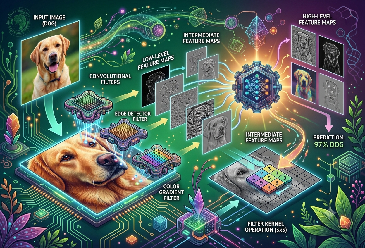
Convolutional Filters & Feature Maps
What Are Filters & Feature Maps?
When you glance at a photo of your dog, your eyes don’t study every pixel one at a time. They get pulled straight toward the things that matter — the edge where an ear meets the head, the dark circle of a nose, the curve of a tail. Convolutional neural networks try to copy that exact trick, and the two tools they use to pull it off are called filters (also known as kernels) and feature maps.
A filter is a tiny window of numbers that slides across an image, searching for one specific pattern. A feature map is the trail it leaves behind — a record of exactly where, and how strongly, that pattern showed up.— A working definition for this guide
In technical terms, a filter is a small two-dimensional grid of learnable weights — numbers the network adjusts during training. Most filters in modern networks are just 3×3 in size, though 5×5 filters show up too. As that tiny grid is dragged across every position of an image, it multiplies its own numbers against the pixels underneath it and adds the results together. Each of those sums lands in a new grid called a feature map (sometimes called an activation map, or a convolved feature) — and that feature map becomes the input the very next layer works with.
Imagine a star-shaped cookie cutter. If you press it down on a big sheet of rolled-out dough and only mark the spots where the star fits, you’ve basically just performed a convolution. The cookie cutter is the filter. The marks left all over the dough are the feature map.
Three Names, Two Ideas
People studying computer vision tend to use a handful of overlapping words for the same two concepts. It helps to untangle them early:
A small grid of learnable numbers — the “lens” that scans the image looking for one particular pattern, like a curved edge or a patch of red.
The grid of results left behind after a filter finishes scanning — the “photograph” taken through that lens, showing where the pattern was strongest.
The mathematical sliding-multiply-and-add operation that turns a filter and an image into a feature map. It’s the verb connecting the two nouns.
It’s worth being precise about one more distinction that trips people up: a feature map is not quite the same thing as an embedding. A feature map keeps its spatial shape — it still has a height and a width that line up with the original image — while an embedding is usually flattened into a single long list of numbers that throws spatial position away in exchange for a compact summary. Feature maps are for “what’s where”; embeddings are for “what’s this, overall.”
Why CNNs See Images Differently
Before convolutional networks took over computer vision, engineers tried feeding images into the same kind of network used for things like predicting house prices — a densely connected, fully-connected network. For images, that approach ran into trouble almost immediately.
A fully-connected network treats every single pixel as its own separate input. A modest color photo of 224×224 pixels with three colour channels already contains 150,528 individual numbers. Connect that to even a few modest hidden layers and the number of trainable weights can balloon into the hundreds of billions before the network has learned anything useful at all. Training a model that large is painfully slow, and with so many free parameters relative to the amount of training data available, it tends to memorize the training images rather than learning anything that generalizes.
There’s a second, sneakier problem: fully-connected networks have no built-in sense of position. If the exact same object shifts a few pixels to the left in a photo, a dense network may treat the shifted image as something completely unfamiliar, because a different set of input neurons is now “lit up.” Convolutional networks solve both problems with one elegant trick: instead of learning a separate rule for every pixel location, they learn one small filter and reuse it — sliding it across every part of the image. This is called parameter sharing, and it’s the single biggest reason CNNs are practical at all.
Why Plain Networks Struggle With Images
- Treats every pixel as an unrelated input
- Parameter count explodes for realistic image sizes
- No built-in tolerance for shifted or moved objects
- Easily overfits with so many free weights
How Convolution Fixes It
- Learns one small filter, reused everywhere (parameter sharing)
- Dramatically fewer trainable weights for the same image
- Pattern detection becomes naturally position-tolerant
- Less prone to memorizing noise instead of patterns
Imagine trying to recognise your best friend by memorising the exact colour of every single hair and freckle on their face, one by one. If they tilt their head just slightly, you’d be totally confused! A CNN instead learns a general rule — like “two eyes above a nose, with a mouth below” — and that rule still works no matter where in the picture your friend’s face happens to be.
The Convolution Operation, Step by Step
Strip away the jargon and a convolution is really just repeated multiplication and addition, performed in a small moving window. Here is exactly what happens, one step at a time.
- The filter is placed over a small patch of the input — this patch is called the receptive field, and for a 3×3 filter it’s simply a 3×3 block of pixels.
- Every one of the filter’s nine numbers is multiplied by the pixel value sitting directly beneath it.
- All nine of those products are added together into a single number — this is the dot product.
- That single number is written into the matching cell of the new feature map.
- The filter then slides over by a fixed number of pixels (the stride) and the whole process repeats.
- Once the filter reaches the end of a row, it drops down to the next row and starts again from the left, until the entire image has been scanned.
A feature map is really just a grid of “match scores.” A high number means the pattern the filter is hunting for showed up strongly at that spot. A low or negative number means it mostly didn’t.
Stride, Padding & Output Size
Three quiet little settings decide exactly how big and how deep every feature map will turn out to be. Get comfortable with these three and the rest of a CNN’s architecture starts to make sense at a glance.
| Hyperparameter | What It Controls | Typical Setting |
|---|---|---|
| Stride | How many pixels the filter jumps after each step | 1, occasionally 2 |
| Padding | Whether extra zeros are added around the input’s border | “Valid”, “Same”, or “Full” |
| Number of filters | How many separate feature maps come out (the output’s depth) | 32 – 512, growing deeper into the network |
The Three Flavours of Padding
No padding at all. The filter only ever sits fully inside the image, so the output shrinks a little with every convolution.
Just enough zeros are added around the border that the output keeps the exact same height and width as the input.
Even more zeros are added, letting the filter sweep past every edge completely — the output actually grows larger than the input.
For an input of width W, a filter of size F, padding P, and stride S, the resulting feature map’s width is: O = ⌊(W − F + 2P) / S⌋ + 1. Worked example: a 32×32 input with a 3×3 filter, one pixel of padding, and a stride of 1 gives O = ⌊(32 − 3 + 2)/1⌋ + 1 = 32 — the spatial size is fully preserved.
Stride is like deciding how big your hops are when crossing stepping stones in a stream. Small hops let you explore every inch closely. Big hops get you across faster but you skip some details. Padding is like adding a couple of pretend stones right at the edge of the stream, so you don’t accidentally fall in the water when you reach the bank.
Multiple Filters, Multiple Maps
A single filter can only ever look for one thing. Real convolutional layers stack dozens — sometimes hundreds — of filters side by side, each hunting for something a little different, and pile their outputs into one tall block of feature maps.
This matters because the number of filters in a layer directly decides the depth of its output. Three different filters produce three separate feature maps, which are stacked together into an output volume that is three layers deep. There’s one strict rule every filter has to obey, though: the depth of a filter must always match the depth of whatever it’s scanning. A filter looking at a colour image with red, green, and blue channels needs a depth of three, with one 3×3 “slice” — called a kernel — for each colour channel. A filter scanning the output of an earlier layer with 64 channels needs a depth of 64 to match.
The other half of the magic is parameter sharing: the same nine weights inside a 3×3 filter are reused at every single position as it slides across the entire image, rather than learning a fresh set of weights for every pixel location. This is precisely why CNNs need so many fewer trainable parameters than a fully-connected network would for an image of the same size, and why a pattern learned in one corner of an image is automatically recognised everywhere else too.
64 filters, each sized 3×3×3 to match the RGB input, add up to roughly 1,792 trainable weights and biases for the entire layer.
For a depth-3 input scanned by two 3×3 filters, that’s 27 weights per filter — 54 weights total, plus one bias per filter, for 56 trainable parameters.
Classic Filters: Edges, Blur & Sharpen
Long before neural networks existed, image-processing engineers hand-designed filters to find edges, soften photos, or sharpen them. A CNN never needs to be told which filters to use — it discovers similar (and sometimes much stranger) ones automatically during training — but seeing a few hand-crafted classics makes the whole idea click immediately.
| Classic Filter | Pattern It Highlights | Typical Use |
|---|---|---|
| Vertical edge detector | A sudden left-to-right brightness change | Finding the side edges of objects |
| Horizontal edge detector | A sudden top-to-bottom brightness change | Finding the top/bottom edges of objects |
| Blur (averaging) kernel | Smooths out sudden changes | Noise reduction, soft focus |
| Sharpen kernel | Boosts contrast right at edges | Making fine details pop |
This is exactly like the filters in a photo-editing app that make a picture look blurry, super-sharp, or “outline only.” The difference is that a CNN doesn’t wait for an engineer to design these filters by hand — it invents its own, through thousands of rounds of trial and error during training.
And here’s the satisfying part: when researchers peek inside the very first convolutional layer of a trained network like VGG16 and plot its filters as little grayscale images, many of them really do look like simple gradient and edge detectors — almost identical in spirit to the hand-designed kernels above. The network rediscovered, on its own, ideas that image-processing engineers had worked out decades earlier.
Activation Maps & the Role of ReLU
A freshly computed feature map is just a grid of plain numbers — some positive, some negative, some sitting right at zero. Before it gets handed to the next layer, almost every CNN pushes that grid through an activation function. Strictly speaking, the result of that step is called an activation map, though in everyday conversation people often use “feature map” loosely for both the raw and the activated version.
The activation function used most often by far is ReLU — short for Rectified Linear Unit. Its rule could not be simpler: keep every positive value exactly as it is, and replace every negative value with zero. That simple snap introduces something a stack of pure convolutions could never produce on its own — non-linearity. Without it, no matter how many convolutional layers were stacked together, the entire network would mathematically collapse into nothing more than one giant linear operation, incapable of learning the curved, complicated decision boundaries that real-world recognition tasks demand.
Zeroes out negative values and leaves positives untouched. Fast to compute, encourages sparse activations, but can suffer from “dead” neurons that never fire again.
Most CommonSquashes every value into the range 0 to 1. Useful for binary outputs, but prone to the vanishing-gradient problem in deep stacks.
BoundedSquashes values into the range −1 to 1. Has a steeper gradient than sigmoid, which can help training, but still faces vanishing gradients in very deep networks.
CenteredConvolution finds patterns. Activation decides which of those findings are worth passing along. Together, they’re the one-two punch repeated, layer after layer, throughout the entire network.
Pooling: Shrinking Without Losing the Point
Feature maps can pile up fast, both in number and in size. Pooling layers step in right after activation to shrink them down, without throwing away the most important signal hiding inside.
A pooling filter slides across the input just like a convolutional filter does — but it carries no learnable weights at all. Instead, at every position it simply applies a fixed aggregation rule to whatever values fall underneath it.
Keeps only the single largest value found inside each small window, discarding the rest. This is the more commonly used technique, since it preserves the strongest signal a filter detected.
Keeps the average of all the values inside each window instead of just the peak, producing a smoother — but slightly less sharp — summary of the feature map.
| Benefit of Pooling | Why It Helps |
|---|---|
| Fewer parameters downstream | Smaller feature maps mean less compute and faster training |
| Tolerance to small shifts | A feature shifted by a pixel or two still gets captured in the same pooled window |
| Reduced overfitting risk | Compressed maps carry less opportunity to memorise noise |
Imagine summarising a long comic book by keeping only the single most exciting panel from every page. You lose a lot of small detail, but you keep the best, most important part. That’s basically what max pooling does to a feature map.
The Feature Hierarchy: From Edges to Objects
Stack enough convolution-activation-pooling blocks together, one after another, and something remarkable happens: the feature maps stop looking like simple lines and start looking like entire object parts — and then, eventually, whole objects.
A landmark 2013 paper on visualizing convolutional networks demonstrated this hierarchy directly. The researchers built a technique to reconstruct, pixel by pixel, exactly which input patches caused the strongest activation in different feature maps throughout a trained network. Early-layer filters, they found, responded mostly to simple edges and patches of colour. Filters several layers deeper responded to far more complex, compositional structures — recognisable parts of objects rather than raw geometry.
There’s a helpful way to picture why this happens. Think of an everyday object — say, a bicycle — as a sum of its parts: a frame, two wheels, handlebars, pedals. Each individual part forms a relatively low-level pattern that an early-to-middle layer can pick up on its own. Combine several of those parts together in the right arrangement, and a much later layer can recognise the higher-level pattern they form together: a bicycle, sitting whole, in the photograph.
Each additional layer effectively “sees” a larger area of the original image, because its receptive field is built from the combined outputs of everything beneath it. That’s the real reason deep networks tend to outperform shallow ones on vision tasks: depth is what lets a network climb from pixels, to patterns, to genuine understanding.
Seeing Inside the Network
CNNs are sometimes called “black boxes,” but they’re more transparent than people assume — researchers have developed two simple, complementary ways to actually open one up and look.
Plot the Filter Weights
Because a filter is just a small 2-D grid of numbers, it can be drawn directly as a tiny grayscale image. Bright squares mark strong (excitatory) weights; dark squares mark weak or inhibitory ones — this shows what a layer is looking for.
Plot the Feature Maps
Run one real photograph through the network and capture the output at a chosen layer. Each channel can be drawn as its own little image, showing exactly where, in that specific photo, the corresponding pattern was detected.
Class Activation Maps
A more advanced relative of feature-map plotting, this technique highlights precisely which pixels of an input image most influenced the network’s final decision — useful for sanity-checking what a model has actually learned.
Researchers experimenting with a well-known pretrained network like VGG16 typically find a consistent, almost reassuring pattern: feature maps pulled from layers close to the input retain a lot of fine detail — recognisable outlines, textures, the rough silhouette of whatever was photographed. Feature maps pulled from layers near the output, on the other hand, look increasingly abstract and blocky, trading recognisable shape for compressed, high-level meaning. By the final convolutional block, a human glancing at the raw feature maps usually can’t tell what object the network saw anymore — yet the network can still classify it correctly, because it isn’t looking for a picture any more. It’s looking for a pattern of numbers that has, time and again, meant “this is a bird” or “this is a bicycle.”
“A filter tells you what the network is looking for. A feature map tells you exactly where it found it.”
— A practitioner’s rule of thumbPros & Cons of Convolutional Feature Extraction
Filters and feature maps unlocked modern computer vision, but the approach is not without real, practical trade-offs that every team building with CNNs eventually runs into.
Pros
- Learns useful features automatically — no manual feature engineering required
- Far fewer trainable parameters than a fully-connected network, thanks to parameter sharing
- Naturally tolerant of small shifts and distortions, thanks to pooling and shared weights
- Builds a genuine hierarchy, capturing both fine detail and big-picture concepts
- Filters learned on one large dataset often transfer well to closely related tasks
Cons
- Computationally demanding — training at scale usually requires a GPU
- Large stacks of feature maps can consume substantial memory
- Deeper layers become genuinely hard to interpret — the “black box” problem
- Needs large amounts of labelled training data to perform well
- Can overfit without enough regularisation, and is sensitive to adversarial noise
Real-World Applications
Once trained, the filters and feature maps inside a CNN aren’t just an academic curiosity — they quietly power a huge slice of the visual technology people interact with every single day.
Healthcare
Early feature maps highlight bone outlines and tissue boundaries in X-rays and MRI scans; deeper maps help flag abnormalities such as tumours, assisting radiologists with diagnosis.
Autonomous Vehicles
Onboard cameras feed CNNs that distinguish lane markings, pedestrians, and traffic signs in real time — a core safety layer behind modern driver-assistance features.
Retail & E-Commerce
Visual search tools use feature maps to find products that look similar to a photo a shopper uploads, recommending items that match a style or pattern.
Security & Identity
Facial-recognition and surveillance systems lean on hierarchical feature maps to identify faces and objects consistently across different angles and lighting.
Agriculture
Drone and field-camera imagery is scanned by CNNs trained to spot early signs of crop disease or stress, well before the naked eye would notice.
Social Media
Auto-tagging suggestions and content recommendations on photo-sharing platforms rely on the very same convolutional feature extraction described in this guide.
Famous Architectures & What’s Next
The idea of a small, sliding, learnable filter has powered roughly four decades of computer-vision progress — refined, scaled, and reinvented by a handful of landmark architectures along the way.
Backpropagation Meets Convolution
Yann LeCun successfully applies backpropagation to train a network recognising handwritten zip codes, building on earlier groundwork from Kunihiko Fukushima.
LeNet-5
A lightweight, formative architecture for handwritten-digit recognition, using shared weights efficiently and laying the template that future CNNs would follow.
AlexNet
Wins the ImageNet Large Scale Visual Recognition Challenge by a wide margin, popularising ReLU activations and dropout, and kicking off the modern deep-learning boom.
VGGNet
Demonstrates that stacking simple, uniform 3×3 filters consistently — up to 19 layers deep — is enough to model very complex visual patterns.
ResNet
Introduces residual (“skip”) connections that let information bypass certain layers, finally making it practical to train networks 50, 100, or more layers deep.
Today’s architectures keep building on this same foundation while optimising for different trade-offs. Inception-style modules use small 1×1 convolutions to shrink feature-map depth before applying larger, more expensive filters, squeezing more accuracy out of less compute. Lightweight designs aimed at phones and embedded devices trim filter counts and depth for speed. Even newer vision transformer architectures, which process images quite differently, still often pair with convolutional layers at the front end to do the early, efficient pattern-spotting that filters have always been good at.
No matter how exotic CNN architectures get, the foundational idea in this guide stays exactly the same: a small, learnable filter slides across data, multiplies-and-sums its way into a feature map, and that process is stacked many times over to learn a hierarchy of patterns — from raw pixels, all the way up to genuine visual understanding.
Cheat-sheet style overview covering layers, activation functions, architectures, training tips, and applications.
Step-by-step breakdown of CNN layers with a worked code example, advantages, and limitations.
Practical tutorial on plotting learned filters and feature maps using a pretrained VGG16 model.
Concise glossary entry distinguishing feature maps from filters, embeddings, and activations.
In-depth walkthrough of convolution, stride, padding, receptive fields, and the VGG-16 architecture.
Technical explanation of feature-map computation, sizing formulas, and pros and cons.
Overview of CNN components, ReLU, inception modules, and GPU-accelerated training and inference.
Practical perspective on how filters extract and combine features for downstream classification.
Foundational explainer on how convolutional layers and filters operate within a network.
Comprehensive explainer covering layer types, hyperparameters, padding, and CNN history.
Tutorial-style introduction to CNN building blocks and common use cases.
Accessible explainer on the role and computation of feature maps.
Worked example connecting kernel count directly to feature-map count.
Short-form answer explaining the feature-map concept for newcomers.
Companion explainer covering CNN fundamentals from a machine-learning perspective.
Practitioner walkthrough of how filters interact with images to produce feature maps.