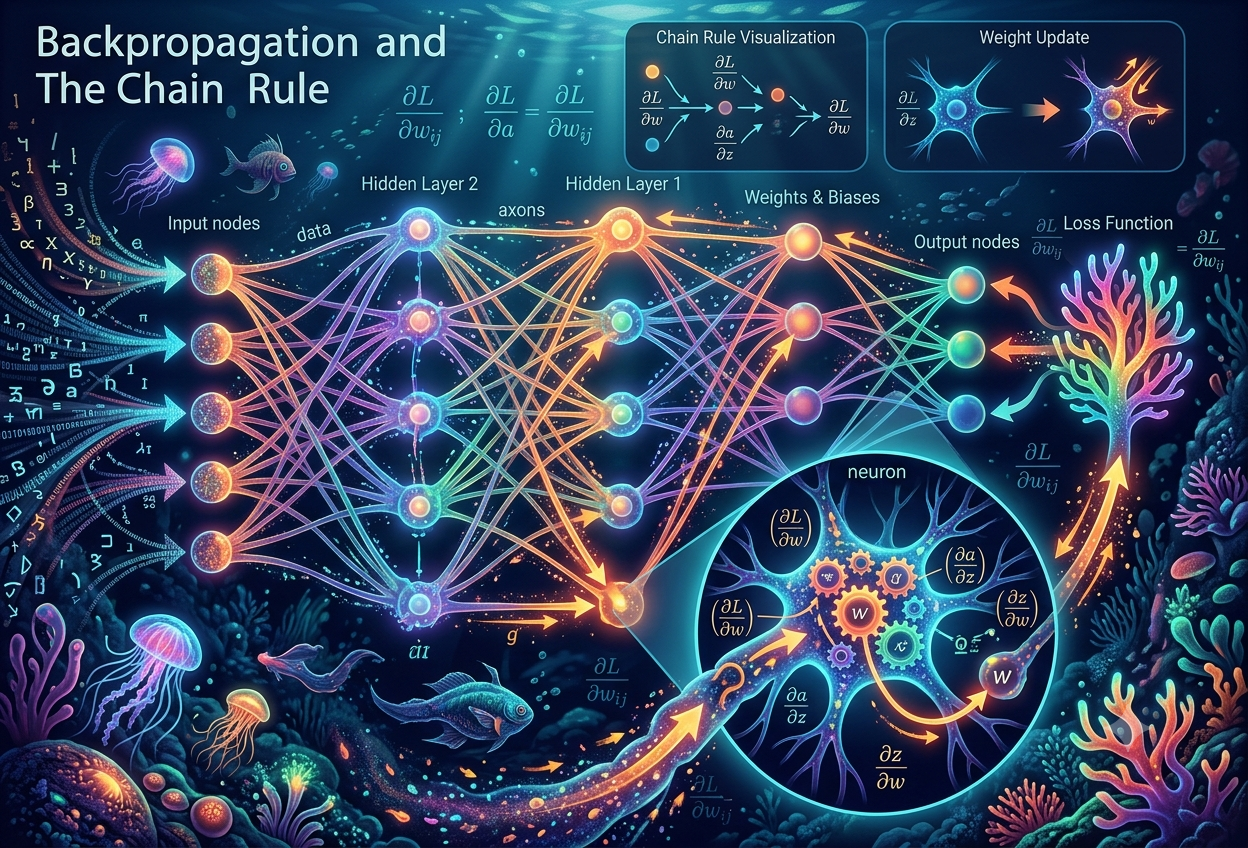
Backpropagation
& The Chain Rule
The algorithm that travels backwards through every layer of a neural network, measures how wrong it was, and tells each weight exactly how to change — built on a single, elegant rule from calculus.
Imagine you throw a dart at a board and miss. You look at where it landed, figure out how far off you were and in which direction, adjust your grip and aim, then throw again. After enough throws, you start hitting the bullseye consistently. That trial-and-error process of adjusting based on feedback is exactly what backpropagation does inside a neural network — except instead of darts, it adjusts millions of numbers called weights, and it learns from patterns in data rather than a physical board.
Backpropagation is the algorithm that teaches a neural network by measuring how wrong its prediction was, then travelling backwards through every layer to figure out how much each weight contributed to that mistake — and by exactly how much each weight should change to do better next time.— Core Concept · Deep Learning Fundamentals
When a neural network makes a prediction, it will almost certainly be wrong at first. The network has to learn from that mistake. Backpropagation is the engine of that learning. It works by calculating a number called the gradient — a precise measure of how much changing each individual weight would improve or worsen the prediction. Once all gradients are known, the weights can be nudged in the right direction, and the network becomes a tiny bit smarter.
The name comes from the direction it travels: it starts at the output (where the mistake was made), then works backwards through every hidden layer until it reaches the inputs. Think of it like a detective working a case backwards — starting at the scene of the crime (the wrong prediction) and tracing every clue back to its source (the individual weights that caused it).
Picture a game of telephone where your message arrives scrambled. Instead of playing forwards again and hoping for better luck, backpropagation rewinds the line and whispers a correction to each player based on exactly how much they garbled the message. After many rounds of corrections, the message travels perfectly. That rewinding and correcting is backpropagation!
Why Backpropagation Matters
Before backpropagation was discovered, researchers had no reliable way to train networks with more than one or two layers. They could build these beautiful multi-layer structures on paper, but could not teach them anything useful. Backpropagation solved this problem completely and sparked the deep learning revolution we live in today.
- It is the universal training algorithm. Every major neural network — from image classifiers to language models — was trained using backpropagation or a direct descendant of it.
- It makes learning mathematically precise. Rather than randomly guessing how to improve, backpropagation computes the exact direction and magnitude of each required adjustment.
- It scales to arbitrary depth. Whether a network has 3 layers or 300, the same algorithm applies — just repeated more times going backwards.
- It is the reason AI works at all. Without backpropagation, we would have no image recognition, no language translation, no speech assistants, and no generative AI.
The chain rule is a rule from calculus — the mathematics of change and rates. It sounds intimidating but the underlying idea is something any ten-year-old intuitively understands. It is simply the rule for figuring out how one thing changes when you change something far down the chain of causes.
The Chain Rule in Plain English
Suppose you are warming up soup on a stove. You turn up the gas (that is your action). The flame gets hotter. The pot gets hotter. Eventually, the soup gets hotter. There is a chain of causes here: gas → flame → pot → soup. If you want to know how much turning up the gas affects the soup temperature, you multiply together how much each link in the chain affects the next.
In mathematics, this chain of causes is expressed as a function inside a function. If soup temperature depends on pot temperature (call that function f), and pot temperature depends on the gas setting (function g), then the combined effect is written as f(g(x)). The chain rule tells us how to differentiate this combination:
where u = g(x) is the intermediate variable (e.g. pot temperature)
and y = f(u) is the final variable (e.g. soup temperature)
In words: “how much y changes per unit x” =
“how much y changes per unit u” × “how much u changes per unit x”
FIG 01 — The chain rule as a pipeline. Each box transforms an input into an output. The total rate of change from x to y is found by multiplying together all the individual rates across every link.
The Chain Rule in Machine Learning
A neural network is nothing more than a very long chain of mathematical functions — one layer after another, each transforming the output of the layer before it. The loss function (the measure of how wrong the network was) sits at the very end of this chain. To improve the network, we need to know how changing any single weight — buried deep inside an early layer — affects that final loss. The chain rule is the only tool powerful enough to compute this across dozens or hundreds of layers.
In a neural network with L layers, the chain rule tells us that the gradient of the loss with respect to a weight in layer 1 is:
∂L/∂W₁ = how much does the loss change if W₁ changes slightly?
∂a_L/∂a_{L−1} = how much does the last layer’s output change if the
second-to-last layer’s output changes? (one link in the chain)
The “…” means we multiply across every single layer between 1 and L
Imagine a row of dominoes. You push the first one (change a weight). It knocks the second, which knocks the third, all the way to the end (the loss value). The chain rule is how you figure out: “If I push the first domino 1 cm harder, how much further does the last one fall?” You multiply together how each domino is pushed by the previous one — across every single domino in the chain.
Assigns precise blame to each weight for the final error. Without it, we would not know which weights to fix.
Instead of testing every weight one at a time (which would take forever), the chain rule computes all gradients in one elegant backwards sweep.
Makes it possible to train networks of any depth. It simply multiplies as many terms as there are layers — 10, 100, or 1000.
A gradient is a signpost. It points in the direction that makes a function increase the most. In neural network training, we want the loss to decrease, so we go in the opposite direction of the gradient — downhill instead of up. This strategy is called gradient descent.
What Is a Gradient?
Imagine you are standing blindfolded on a hilly landscape and you want to find the lowest valley. You cannot see anything, but you can feel the slope under your feet. If the ground tilts downward to your left, you step left. If it tilts forward, you step forward. The gradient is simply the measure of how steeply the ground tilts in each direction, and gradient descent is the strategy of always stepping in the downhill direction.
In a neural network, the “landscape” is the loss surface — an abstract multi-dimensional space where each dimension corresponds to one weight. Moving in this space means changing weights. The goal is to find the lowest point in this landscape: the configuration of weights that minimises the prediction error.
FIG 02 — Gradient descent on a 1D loss surface. Both starting points (red from the left, blue from the right) follow the downhill gradient step-by-step until converging near the global minimum of the loss.
The Learning Rate: Controlling Step Size
During gradient descent, the network does not jump all the way to the minimum in one go — that would overshoot. Instead it takes small, controlled steps. The size of each step is governed by the learning rate (usually written as α, the Greek letter alpha). Choose a step size that is too large and you will bounce right over the minimum. Choose one that is too small and training will take an impossibly long time.
w = the weight being updated
α = learning rate (e.g. 0.01 — a small positive number)
∂L/∂w = gradient — how much the loss changes if w increases slightly
Minus sign: we move OPPOSITE to the gradient (downhill)
Learning Rate Too Large
Steps are too big. The weight update jumps past the minimum and the loss bounces chaotically — training never converges. The network oscillates wildly and may diverge completely.
Learning Rate Too Small
Steps are tiny. The network does improve, but so slowly that it would take millions of extra iterations to reach a good solution. Computationally wasteful in large systems.
Learning Rate Just Right
The loss decreases steadily with each batch of training data. The network converges efficiently. Finding this “Goldilocks” value is a key hyperparameter tuning challenge.
Adaptive Learning Rates
Modern optimisers like Adam, AdaGrad, and RMSProp automatically adjust the learning rate for each weight individually — solving the tuning problem elegantly for most networks.
Backpropagation is not magic — it is a precise four-phase recipe that runs once per training iteration. Let us break it down into every individual step so the whole process becomes as clear as following a cooking recipe.
FIG 03 — The four-phase training cycle. Each complete cycle (called one iteration or step) uses one mini-batch of training data. This cycle repeats thousands or millions of times during training.
- Forward Pass. Feed a batch of training examples through the network from input to output, computing every neuron’s activation along the way. Store these intermediate values — they will be needed during the backward pass. The output is the network’s current prediction ŷ.
- Compute the Loss. Compare ŷ against the true label y using a loss function. The result is a single number L representing how wrong the prediction was. A loss of 0 would be perfect; in practice, loss decreases slowly but steadily during training.
- Backward Pass (Backpropagation). Starting at the output layer, apply the chain rule to compute ∂L/∂W for every weight in every layer. The gradients flow backwards — from output layer to the last hidden layer, then through every hidden layer until reaching the first. All stored intermediate values from the forward pass are used here.
- Update the Weights. Apply the gradient descent update rule to every weight: subtract the gradient multiplied by the learning rate. Now the weights are slightly better than before. One complete forward + backward cycle constitutes a single training step.
The cycle above repeats once per mini-batch. If you have 60,000 training samples and use a batch size of 32, that is about 1,875 steps per epoch (a full pass over the training data). Modern networks often train for 10 to 100+ epochs, meaning they might complete millions of forward-backward cycles before the weights are considered well-trained.
Nothing cements understanding like tracing real numbers through every step. We will build the tiniest possible network — two inputs, one hidden neuron, one output — and watch backpropagation correct a wrong prediction from start to finish.
FIG 04 — A minimal network with real values. The forward pass produces ŷ = 0.654 against a true target of 1.0, giving a loss of 0.060. Dashed red arrow shows the backward direction of gradient flow.
Step-by-Step with Real Numbers
Step 1 — Forward Pass
a = sigmoid(0.88) = 0.707 (the hidden neuron’s output)
ŷ = sigmoid(w₃ × a) = sigmoid(0.9 × 0.707) = sigmoid(0.636) = 0.654
Step 2 — Compute Loss (MSE)
The ½ in front is a mathematical convenience — it cancels when we differentiate later
Step 3 — Backward Pass (Chain Rule in Action)
GRADIENT THROUGH SIGMOID ACTIVATION (sigmoid’ = ŷ × (1 − ŷ)) ∂ŷ/∂z_out = 0.654 × (1 − 0.654) = 0.654 × 0.346 = 0.226
GRADIENT OF LOSS WITH RESPECT TO w₃ — OUTPUT WEIGHT (CHAIN RULE) ∂L/∂w₃ = (∂L/∂ŷ) × (∂ŷ/∂z_out) × a = (−0.346) × 0.226 × 0.707 = −0.0552
Step 4 — Update the Weight
The weight increased slightly — pushing the output closer to 1.0 on the next pass
The network predicted 0.654 when the correct answer was 1.0. Backpropagation computed that w₃ should increase from 0.9 to 0.9055. That tiny bump means the next forward pass will produce a prediction slightly closer to 1.0. Repeat this process thousands of times across all weights and all training examples, and the network gradually becomes accurate.
Before backpropagation can compute any gradient, we need a single number that summarises how wrong the network was. That number comes from the loss function — sometimes called the cost function or objective function. Choosing the right loss function is one of the most important design decisions when building a neural network.
| Loss Function | Formula | Best Used For | Key Property |
|---|---|---|---|
| Mean Squared Error (MSE) | ½(ŷ − y)² | Regression — predicting continuous numbers | Heavily penalises large errors; smooth gradient everywhere |
| Mean Absolute Error (MAE) | |ŷ − y| | Regression when outliers are a concern | More robust to outliers than MSE; gradient is constant magnitude |
| Binary Cross-Entropy | −[y·log(ŷ) + (1−y)·log(1−ŷ)] | Binary classification (yes/no, true/false) | Ideal with sigmoid output; heavily penalises confident wrong predictions |
| Categorical Cross-Entropy | −Σ yᵢ · log(ŷᵢ) | Multi-class classification (cat/dog/bird/…) | Ideal with softmax output; standard loss for language models |
| Huber Loss | MSE if |error| < δ else MAE | Regression with some outliers in data | Best of both MSE and MAE — smooth near zero, robust far out |
| KL Divergence | Σ P(x) log(P(x)/Q(x)) | Variational autoencoders, generative models | Measures how different two probability distributions are |
The loss function is the neural network’s sense of regret. It encodes what we care about — accuracy, confidence, fairness, or efficiency — in a single number that the entire training process works to minimise.
— Core Principle · Neural Network DesignThe forward pass and the backward pass are inseparable partners. One cannot exist without the other during training. Understanding the difference between them — and how they interlock — is essential for understanding how neural networks learn.
FIG 05 — The two passes through a neural network during training. Green arrows show data flowing forward during the forward pass. Red arrows show gradients flowing backward during backpropagation.
Forward Pass
Direction: Input → Output. Computes: Activations and final prediction ŷ. Used in: Training AND deployment/inference. Weights are not updated during the forward pass — they are frozen and simply applied.
Backward Pass
Direction: Output → Input. Computes: Gradients ∂L/∂W for every weight, via the chain rule. Used in: Training only — never during live inference. Without this pass, no learning can occur.
Weight Update
When: After every backward pass. What: Each weight is nudged slightly in the direction that reduces loss, using the gradient computed during the backward pass and the current learning rate.
One Epoch
Definition: One complete pass over the entire training dataset — meaning every training example has been seen by the network once. Training typically spans many epochs until the loss stops improving.
Backpropagation is powerful, but it is not immune to problems. Practitioners have spent decades cataloguing the ways it can fail — and developing clever solutions. Understanding these problems is part of what separates a good deep learning engineer from a great one.
In very deep networks, the gradient shrinks as it passes through each layer backwards. By the time it reaches the early layers, the signal is so tiny that the weights there barely update at all — those layers stop learning. Common with sigmoid and tanh activations.
The opposite problem: gradients multiply and grow exponentially as they travel back, eventually producing numbers so large (NaN, infinity) that weight updates become meaningless. Common in recurrent networks processing long sequences. Fixed with gradient clipping.
The loss surface has many valleys. Gradient descent may settle into a small local minimum rather than the best possible global one. In practice, high-dimensional surfaces have more saddle points than local minima, and modern techniques handle this reasonably well.
A saddle point is a location where the gradient is zero but it is neither a minimum nor a maximum — like the centre of a saddle shape. Gradient descent can stall here for many steps. Momentum-based optimisers generally escape these more effectively.
The network memorises the training data rather than learning general patterns. On new, unseen data it performs poorly. Addressed through regularisation (dropout, L2 weight decay), data augmentation, early stopping, and larger or more diverse datasets.
With the ReLU activation, neurons that receive a very negative pre-activation value output 0 permanently — they “die” and produce a zero gradient forever, contributing nothing to learning. Leaky ReLU, PReLU, and ELU activations were created specifically to address this.
Solutions at a Glance
| Problem | Primary Causes | Modern Solutions |
|---|---|---|
| Vanishing Gradients | Deep networks, sigmoid/tanh activations | ReLU activation, batch normalisation, residual connections (ResNets) |
| Exploding Gradients | Deep RNNs, bad weight initialisation | Gradient clipping, proper weight initialisation (Xavier, He) |
| Local Minima / Saddle | Non-convex loss surfaces | Adam optimiser, momentum, learning rate schedules |
| Overfitting | Too few data, too many parameters | Dropout, L1/L2 regularisation, data augmentation, early stopping |
| Dead Neurons | ReLU with bad initialisation or large LR | Leaky ReLU, batch normalisation, careful learning rate tuning |
| Slow Convergence | Fixed or poorly chosen learning rate | Adam, RMSProp, cyclical learning rate schedules |
Every capability of modern AI that impresses or surprises you was built using backpropagation. Without it, none of the neural networks behind these applications could have ever learned to do what they do.
Large Language Models
GPT, Claude, Gemini, LLaMA — every large language model was trained using backpropagation applied to billions or hundreds of billions of parameters over trillions of text tokens. The gradient computations during training consumed enormous amounts of GPU compute over weeks or months, producing models capable of nuanced language understanding and generation.
Image Generation
Diffusion models and GANs (Generative Adversarial Networks) train using backpropagation. The generator and discriminator in a GAN each have their own loss functions, and backpropagation trains both networks simultaneously — a delicate balancing act that produces photorealistic images, videos, and artwork from text prompts.
Reinforcement Learning
When an AI learns to play chess, Go, or video games at superhuman levels, it uses a neural network trained with backpropagation to estimate how valuable any given game state is. AlphaGo, AlphaZero, and OpenAI Five all relied on this combination of reinforcement learning signals fed back through backpropagation.
Drug Discovery
AlphaFold 2, which predicted the 3D structure of nearly every known protein — a 50-year-old grand challenge in biology — used backpropagation to train its neural network. The breakthrough has accelerated drug design, vaccine development, and fundamental research in ways that were unimaginable just a few years ago.
Finance & Trading
Deep neural networks trained via backpropagation analyse market patterns, detect fraudulent transactions, assess credit risk, and generate trading signals. Every major financial institution now uses some form of backpropagation-trained model in its risk and operations pipelines.
Search & Recommendations
When Google ranks search results, YouTube recommends a video, or Spotify suggests a song — deep networks trained by backpropagation are doing the ranking. These systems process your history, preferences, and context through learned embeddings built entirely via backpropagation during training.
✓ STRENGTHS
- Mathematically exact. Backpropagation computes the true gradient of the loss with respect to every weight — not an estimate or approximation. This precision is why it works so reliably across such diverse network architectures.
- Scales to any depth. The same algorithm applies whether the network has 2 layers or 200. Adding depth simply means more chain-rule multiplications during the backward pass.
- Hardware-friendly. The matrix multiplications in backpropagation map perfectly onto GPU and TPU architectures, enabling parallel computation across billions of parameters simultaneously.
- Works with any differentiable architecture. CNNs, RNNs, Transformers, autoencoders — all are trained using backpropagation because all are differentiable systems.
- Enables automatic differentiation. Modern frameworks (PyTorch, JAX, TensorFlow) implement backpropagation automatically — engineers only need to define the forward pass.
- Computationally efficient. A single backward pass computes gradients for all weights simultaneously, rather than perturbing one weight at a time.
✗ LIMITATIONS
- Requires differentiability. Every function in the network must be differentiable (or at least have a useful subgradient). Non-smooth operations — like sorting or selecting the maximum element — cannot be directly backpropagated through.
- Energy and memory intensive. Training large models via backpropagation on enormous datasets requires vast amounts of GPU memory and energy — raising environmental and access-equity concerns.
- No biological plausibility. The human brain does not use anything like backpropagation. Signals in real neurons travel forward, not backward. Backpropagation is an engineering algorithm, not a model of biological cognition.
- Sensitive to hyperparameters. Learning rate, batch size, weight initialisation, and architecture choices all dramatically affect whether backpropagation converges, diverges, or stagnates.
- Produces black-box models. Backpropagation distributes learning across millions of weights in ways that are extremely difficult to interpret.
- Can overfit aggressively. Given enough capacity, a network trained by backpropagation will memorise training data perfectly rather than generalising.
Backpropagation was not invented in a single moment by a single person. It emerged over decades of simultaneous and overlapping discovery — a story of ideas colliding, being forgotten, and then suddenly catching fire when the world was ready for them.
Early Seeds — Control Theory and Automatic Differentiation
Researchers in control theory began developing methods to propagate derivatives backwards through dynamic systems. Henry Kelley (1960) and Arthur Bryson (1961) independently derived gradient computations for control systems — mathematical cousins of what would later become backpropagation, though applied to engineering rather than neural networks.
Linnainmaa — Reverse Mode Automatic Differentiation
Finnish mathematician Seppo Linnainmaa published a method for computing derivatives of composite functions in reverse — essentially the mathematical skeleton of backpropagation. His work, buried in a Finnish Master’s thesis, went largely unnoticed in the neural network community for over a decade.
Werbos — First Application to Neural Networks
Paul Werbos, in his Harvard PhD thesis, explicitly described applying reverse-mode differentiation to train neural networks — the clearest precursor to modern backpropagation. Tragically, his work was largely overlooked, partly because the deep learning community did not yet exist in any meaningful form.
Rumelhart, Hinton & Williams — The Landmark Paper
“Learning representations by back-propagating errors” was published in Nature by David Rumelhart, Geoffrey Hinton, and Ronald Williams. This paper is widely considered the birth of practical deep learning. It demonstrated, with clarity and rigour, that multi-layer networks could learn complex representations when trained with backpropagation — something previously thought impossible. A second AI winter was averted.
LeCun Applies Backprop to Convolutional Networks
Yann LeCun demonstrated that backpropagation could train convolutional neural networks — networks designed to process images using spatially-aware filters. His system read handwritten digits on cheques for US banks with near-human accuracy, the first large-scale commercial AI application of backpropagation.
AlexNet and the GPU Revolution
Alex Krizhevsky, Ilya Sutskever, and Geoffrey Hinton trained a deep convolutional network called AlexNet using backpropagation on GPUs, crushing the ImageNet competition by a margin that stunned the computer vision community. The insight was simple but transformative: backpropagation had always worked — it just needed faster hardware. The deep learning era officially began.
Automatic Differentiation Frameworks Mature
PyTorch (2017) and TensorFlow 2.0 (2019) made automatic differentiation — backpropagation under the hood — accessible to any engineer who could write Python. The democratisation of backpropagation sparked an explosion in research and commercial AI applications that continues today. The algorithm no longer required mathematical expertise to deploy.
Trillion-Scale Backpropagation
Training runs for GPT-4, Gemini Ultra, and other frontier models consumed thousands of GPU-years and performed backpropagation across hundreds of billions of parameters over trillions of data tokens. The algorithm that began in a Finnish Master’s thesis now runs at civilisational scale.
Backpropagation has powered AI for nearly four decades. But researchers are actively exploring whether there are better, cheaper, or more brain-like alternatives — and whether the limitations of backpropagation can be systematically overcome.
Forward-Forward Algorithm
Geoffrey Hinton (2022) proposed the Forward-Forward algorithm — training using two forward passes (one with “good” data, one with “bad”) instead of a backward pass. Early results are promising and it avoids several problems with traditional backprop.
Local Learning Rules
Researchers are developing learning algorithms where each neuron updates based only on local information — no global backward pass needed. This is more biologically plausible and would enable training on neuromorphic (brain-inspired) hardware.
Efficient Sparse Backprop
As models grow larger, computing gradients for every parameter becomes prohibitively expensive. Techniques like gradient checkpointing, mixed-precision training, and selective weight freezing are making backpropagation feasible at trillion-parameter scale.
Quantum Backpropagation
Theoretical work on quantum neural networks proposes quantum circuit analogs of backpropagation that could compute gradients exponentially faster for certain problem types — though practical quantum hardware capable of running these remains years away.
Greener Training
The enormous energy cost of running backpropagation on large models is driving research into more efficient training regimes — curriculum learning, better data curation, distillation, and architectural efficiencies that reduce the number of backward passes needed.
Interpretable Gradients
Techniques like gradient-weighted class activation mapping (Grad-CAM) use the gradients produced during backpropagation to generate explanations for what a model has learned — an emerging field that uses backprop not just for training but for transparency.
Backpropagation and the chain rule together form the mathematical engine behind every neural network that has ever learned anything. The chain rule lets us compute how changing any weight in any layer affects the final loss — no matter how many layers lie between them. Backpropagation uses those computed gradients to update every weight simultaneously, nudging the network closer to correct predictions with each iteration. Done millions of times, across terabytes of data, this simple cycle of predict → measure error → propagate backwards → update → repeat is what allows machines to learn to see, speak, reason, and create. It is, without any hyperbole, one of the most consequential algorithms in human history.
Backpropagation is the algorithm that trains neural networks by computing gradients of the loss function with respect to every weight, using the chain rule of calculus. The chain rule multiplies rates-of-change across every layer, efficiently attributing blame for the prediction error back to every individual weight. Gradient descent then uses these gradients to nudge each weight slightly in the direction that reduces the loss. This complete cycle — forward pass → loss → backward pass → weight update — repeats thousands to millions of times until the network learns to make accurate predictions. Problems like vanishing gradients, exploding gradients, and overfitting challenge practitioners, but decades of research have produced powerful tools to address each one.
Quantitative finance-focused overview of backpropagation covering the algorithm mechanics, weight updates, and practical implementation in trading systems.
Step-by-step technical explanation of how the chain rule is applied layer-by-layer during gradient computation in neural network training.
Mathematical treatment of the chain rule in the context of automatic differentiation and deep learning, with worked examples.
Algorithms-focused walkthrough of how the chain rule enables gradient computation for multi-layer networks, with diagrams and numerical examples.
Deep technical blog post tracing how information and gradients flow through neural networks, with a rigorous mathematical perspective from a systems researcher.
Comprehensive encyclopaedic reference covering the history, mathematical formulation, variants, and academic reception of backpropagation across 60+ years.
Enterprise-level explainer on backpropagation’s role in AI systems, its relationship to gradient descent, and how it fits into the broader neural network training pipeline.
Practical guide to the chain rule focused on its role in quantitative finance machine learning models, with intuitive analogies and numerical examples.
Accessible narrative explainer connecting the chain rule of calculus to the mechanics of backpropagation, with beginner-friendly analogies and visual intuition.
Complete technical tutorial covering the forward pass, loss computation, backward pass, and weight update steps with worked numerical examples and Python code.