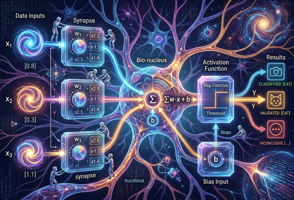
The Perceptron — The Simplest Neural Unit
What Is a Perceptron?
Imagine a tiny robot judge whose only job is to answer yes-or-no questions. You hand it a few clues, it weighs how important each clue is, adds everything up, and shouts either “YES!” or “NO!” That tiny judge is a perceptron — the smallest, simplest thinking unit in all of artificial intelligence.
A perceptron is the simplest kind of artificial neuron: it takes several number inputs, multiplies each one by an importance score called a weight, adds them together with a nudge called a bias, and fires a 1 or a 0 depending on whether the total crosses a threshold.— Working Definition
In technical language, the perceptron is a binary linear classifier. Let’s unpack those three words slowly. Binary means it can only choose between two answers — like spam or not-spam, cat or not-cat, pass or fail. Linear means the invisible wall it draws between the two groups is always perfectly straight — a line in 2D, a flat plane in 3D, and a “hyperplane” in higher dimensions. Classifier means its entire job is sorting things into categories.
Despite being almost 70 years old, the perceptron is still the very first thing taught in nearly every machine learning course on Earth. Why? Because every gigantic neural network powering today’s chatbots, image generators, and self-driving cars is — at its core — millions of slightly upgraded perceptrons wired together. Understand this one little unit, and you hold the master key to understanding all of deep learning.
Pretend you’re deciding whether to play outside. You check three clues: Is it sunny? Did you finish homework? Is your best friend free? But not all clues matter equally — maybe the friend matters most (weight = 3), homework matters a bit (weight = 2), and sun matters least (weight = 1). You add up the points from the clues that are true. If the total beats your “excitement threshold,” you grab your shoes and run outside. Congratulations — your brain just acted exactly like a perceptron!
Three Names You Might Hear
Different books describe the same little machine using different vocabulary. They all point to the same idea:
Emphasises the biological inspiration — a simplified mathematical copy of a brain cell that “fires” when stimulated enough.
Emphasises the mechanics — combine inputs in a straight-line (linear) way, then check the total against a threshold.
Emphasises the architecture — it’s a neural network with exactly one layer of computation and zero hidden layers.
Why the Perceptron Matters So Much
Before 1958, every computer on Earth did exactly — and only — what a human programmer typed into it, step by step. The perceptron shattered that idea. For the first time in history, a machine improved itself by studying examples instead of obeying hand-written rules.
This was a genuine revolution in how people thought about computation. Earlier pattern-recognition systems forced engineers to anticipate every possible situation and write an explicit rule for it. Want to recognise handwritten digits? You’d have to manually code rules about loops, straight strokes, and curves — then debug each rule by hand, forever. The perceptron flipped the workflow: instead of writing rules, you simply show the machine labelled examples, and it discovers the patterns on its own by adjusting its internal importance scores.
“Don’t code the answer — train on the data.” That single shift in mindset, born with the perceptron, is the seed from which all of modern machine learning grew.
The core philosophy of machine learningFour Reasons It Still Matters Today
Every modern deep network — vision models, language models, recommendation engines — is built by stacking and connecting upgraded versions of this single unit.
Weights, bias, activation, training loops, learning rate — every core ML concept appears here in its simplest possible form, making it the ideal first lesson.
It comes with an actual proof (the convergence theorem) guaranteeing it will find a solution whenever a straight-line answer exists. Few algorithms offer such certainty.
For simple, cleanly separable yes/no problems on tiny devices, a perceptron remains a fast, memory-friendly, perfectly respectable choice even now.
Old computers were like a cook who can only follow a recipe word-for-word — change one ingredient and they panic. The perceptron was the first cook who could taste the soup and fix it. Too salty? Add water. Too bland? Add spice. It learns by tasting its own mistakes. That’s why it was such a big deal!
A Short History: Triumph, Winter, and Rebirth
The perceptron’s life story reads like a movie: a dazzling debut, wild promises, a devastating critique, decades in the wilderness, and finally a triumphant return as the ancestor of all modern AI.
The story begins in 1943, when a neuroscientist named Warren McCulloch and a logician named Walter Pitts published a mathematical model showing that simplified brain cells could, in theory, compute logical statements. Their neuron was clever but frozen — it couldn’t learn or change. Fifteen years later, psychologist Frank Rosenblatt, working at the Cornell Aeronautical Laboratory in Buffalo, New York, added the missing magic ingredient: a training rule that let the neuron adjust itself from experience.
Rosenblatt’s project was funded by the United States Navy during the Cold War, when the military badly wanted machines that could spot aircraft, ships, and tanks in aerial photographs without armies of human analysts. In 1958 he first simulated the perceptron in software on an IBM 704 — a room-sized computer — and then built dedicated hardware called the Mark I Perceptron: a camera with a 20×20 grid of 400 light-sensing photocells, whose connection strengths were stored in physical knobs (potentiometers) turned by small electric motors during learning. It learned to tell simple shapes and letters apart.
The 1958 press coverage was, to put it mildly, enthusiastic. Newspapers breathlessly suggested the device was the embryo of a future computer that might one day see, speak, walk, and even reproduce itself. Rosenblatt’s genuine optimism plus media excitement set expectations sky-high — which made the crash that followed feel all the more brutal. A lesson the AI field has had to relearn several times since!
The McCulloch–Pitts Neuron
The first mathematical model of a brain cell as a logic device. Brilliant, but it had fixed connections — it could compute, yet never learn.
Hebb’s Learning Idea
Psychologist Donald Hebb proposed that brain connections strengthen when neurons fire together — often summarised as “cells that fire together, wire together.” This planted the seed for weight-based learning.
Rosenblatt’s Perceptron Is Born
At Cornell Aeronautical Laboratory, Frank Rosenblatt creates the first artificial neuron that genuinely learns from examples, first in software, then as the Mark I hardware machine.
The Convergence Proof
Rosenblatt publishes “Principles of Neurodynamics,” including a proof that the perceptron is mathematically guaranteed to find a correct answer whenever the data can be split by a straight line.
Minsky & Papert Drop the Hammer
MIT researchers Marvin Minsky and Seymour Papert publish the book “Perceptrons,” rigorously proving that a single perceptron can never solve certain simple problems — most famously XOR. Funding dries up almost overnight.
The First AI Winter
Neural network research enters a long freeze. Money, students, and attention flow elsewhere. Tragically, Rosenblatt dies in a boating accident in 1971, never seeing his idea vindicated.
Backpropagation Revives the Field
Rumelhart, Hinton, and Williams popularise backpropagation, a method for training multi-layer networks — exactly the architecture Minsky and Papert said was needed but couldn’t yet be trained. The winter thaws.
The Deep Learning Explosion
Massive datasets and graphics-card computing power let researchers stack millions of perceptron-style units into deep networks, igniting the modern AI era — from image recognition to large language models.
Think of the perceptron like the very first bicycle ever built. At first everyone screamed “This will replace cars and planes!” Then someone pointed out a bicycle can’t fly, and everyone got sad and stopped riding for twenty years. Later, inventors connected the bicycle’s best ideas into motorcycles and engines — and suddenly the old bicycle was a hero again, because everything new was built from its parts.
The Brain Cell Behind the Idea
Rosenblatt didn’t dream up the perceptron from thin air — he copied nature’s homework. Your brain contains roughly 86 billion neurons, and each one works surprisingly like a tiny voting machine.
A biological neuron receives chemical-electrical signals through branching tendrils called dendrites. Some incoming signals are encouraging (“fire!”) and others are discouraging (“stay quiet!”). The cell body adds all these pushes and pulls together, and if the combined excitement crosses a tipping point, the neuron fires — shooting an electrical pulse down its long cable, the axon, toward thousands of downstream neurons. If the excitement falls short, nothing happens at all. It’s an all-or-nothing event, exactly like the perceptron’s 1-or-0 output.
| Biological Neuron | Perceptron Equivalent | Job |
|---|---|---|
| Dendrites | Inputs (x1, x2, … xn) | Carry incoming signals into the unit |
| Synapse strength | Weights (w1, w2, … wn) | Decide how loudly each signal is heard |
| Cell body (soma) | Summation (Σ) | Add all weighted signals together |
| Firing threshold | Bias + step function | Decide whether the total is enough to fire |
| Axon output | Output (0 or 1) | Send the final decision onward |
A brain cell is like a kid standing in a swimming pool with friends splashing water at them. Little splashes? The kid just stands there. But when enough friends splash at once and the water goes over the kid’s nose — SPLASH BACK! All or nothing. The perceptron copies this: small total, stay quiet (0); big total, fire away (1).
Real neurons are enormously more complicated than perceptrons — they use chemistry, precise timing, and thousands of connection types that the math version completely ignores. The perceptron is to a real neuron what a stick figure is to a real human: inspired by it, useful for explaining, but nobody should confuse the two.
Anatomy of a Perceptron
A perceptron is built from exactly five parts. Learn these five, and you’ve learned the vocabulary of every neural network that has ever existed.
Part 1 — Inputs: The Clues
Inputs (written x1, x2, … xn) are the numerical facts you feed the perceptron about one example. For an email spam detector, the inputs might be: how many times the word “FREE” appears, whether the sender is a stranger, and how many exclamation marks the message has. On their own, inputs are just raw numbers waiting to be interpreted — they have no influence until a weight gives them a voice.
Part 2 — Weights: The Importance Scores
Each input gets its own weight (w1, w2, … wn), a number expressing how much that clue should sway the decision. A large positive weight means “this clue strongly pushes toward YES.” A large negative weight means “this clue strongly pushes toward NO.” A weight near zero means “ignore this clue, it barely matters.” The crucial point: weights are the part the perceptron learns. Training is nothing more than the slow, patient adjustment of these numbers.
Part 3 — Bias: The Head Start (or Handicap)
The bias (b) is a single extra number added to the total no matter what the inputs say. Think of it as the perceptron’s built-in mood. A big positive bias makes it trigger-happy — eager to shout YES even with weak evidence. A big negative bias makes it stubborn — demanding overwhelming evidence before firing. Geometrically, the weights tilt the decision line while the bias slides it around; without a bias, the line would be forced to pass through the origin point (0,0), badly limiting what the perceptron could separate.
Part 4 — The Weighted Sum: Adding It All Up
The perceptron multiplies each input by its weight, adds the results, and tops it off with the bias. This single number, usually called z, represents the total strength of evidence. The bigger z is, the louder the inputs are screaming “YES!”
Part 5 — The Activation (Step) Function: The Final Judge
Finally, the step function looks at z and makes the call: if z is zero or higher, output 1; otherwise, output 0. No maybes, no percentages, no shades of grey — a hard, instant verdict. This sudden jump from 0 to 1 is why it’s drawn as a “step,” and it directly mimics the all-or-nothing firing of a real neuron.
Picture a talent show with three judges (inputs). One judge is famous, so her vote counts triple (big weight). One judge is new, so his vote counts once (small weight). The host also secretly loves the contestant and adds 2 bonus points before anyone votes (bias). Add up all the points (weighted sum). If the total reaches 10, the golden buzzer fires (step function) and the contestant goes through (output = 1)!
The Math, Made Friendly
Two short formulas describe everything a perceptron does. If you can multiply and add, you can master both of them right now.
Formula 1 — Computing the Total Evidence
In compact mathematical notation this is written z = Σ wi·xi + b, where the big Greek letter Σ (sigma) simply means “add up all of these.” Vector lovers write it even shorter as z = w·x + b, using the dot product. All three notations mean the identical thing: multiply pairs, then sum.
Formula 2 — Making the Decision
The symbol ŷ (pronounced “y-hat”) means “the predicted answer,” as opposed to plain y, which is the true answer from the training data. Comparing ŷ against y is how the perceptron discovers it made a mistake.
Wait — Where Did the Threshold Go?
Older textbooks describe the rule as “fire if the sum exceeds some threshold θ (theta).” Modern notation hides the threshold inside the bias: requiring (sum ≥ θ) is exactly the same as requiring (sum − θ ≥ 0), so we just define b = −θ and always compare against zero. Same machine, tidier bookkeeping — and it means the threshold becomes a learnable number like any weight.
The math is just a lemonade-stand calculation. Cups sold × price per cup, plus tips jar (bias) = today’s money (z). If the money is enough to buy the video game (z ≥ 0 after subtracting the game’s cost), you celebrate (output 1). If not, you don’t (output 0). You already do perceptron math every day!
How a Perceptron Makes a Decision
Let’s run one complete decision in slow motion. The question: “Should I go to the park?” Our perceptron checks three clues and weighs each by how much it cares.
The Setup
| Clue (Input) | Today’s Value | Weight (Importance) | Contribution |
|---|---|---|---|
| Is it sunny? (x1) | 1 (yes) | w1 = 2.0 | 1 × 2.0 = 2.0 |
| Is homework done? (x2) | 0 (no) | w2 = 3.0 | 0 × 3.0 = 0.0 |
| Is my friend free? (x3) | 1 (yes) | w3 = 4.0 | 1 × 4.0 = 4.0 |
| Bias (built-in laziness) | — | b = −5.0 | −5.0 |
The Calculation
z = 2.0 + 0.0 + 4.0 + (−5.0) = 1.0
Since z = 1.0 is greater than or equal to zero, the step function fires: ŷ = 1 → GO TO THE PARK!
Notice the elegance: the unfinished homework (the most heavily weighted “no”) nearly killed the trip, and the negative bias means this perceptron needs real convincing. But sunshine plus a free friend together supplied just enough evidence to tip the verdict. Change any one number and the answer can flip — that sensitivity to weights is exactly what training will exploit.
This forward pass — inputs in, weighted sum, nonlinearity, output — is exactly the computation performed billions of times per second inside modern GPUs running deep networks. Today’s neurons swap the harsh step function for smoother curves (sigmoid, tanh, ReLU), but the skeleton of the computation is unchanged since 1958.
How a Perceptron Learns
Here is the perceptron’s superpower — the part that made history. It learns from its mistakes using one beautifully simple rule: when wrong, nudge the weights in the direction that would have made you right.
The Learning Loop, in Plain Words
- Start clueless. Set all weights and the bias to zero (or small random numbers). The perceptron knows nothing yet.
- Show one training example. Feed in its inputs and let the perceptron predict ŷ using the current weights.
- Compare with the truth. Compute the error: (y − ŷ). If the prediction was correct, the error is 0 — touch nothing and move on.
- If wrong, nudge. Adjust every weight a little: wi ← wi + η·(y − ŷ)·xi, and nudge the bias too: b ← b + η·(y − ŷ).
- Repeat for all examples. One full sweep through the training data is called an epoch.
- Keep looping epochs until a full pass produces zero mistakes (or you hit your patience limit).
Why This Rule Is So Clever
Look at what (y − ŷ) can be. If the true answer was 1 but the perceptron said 0, the error is +1 — so the rule increases the weights of any active inputs, making the perceptron more likely to fire next time on similar evidence. If the truth was 0 but it said 1, the error is −1 — weights of active inputs get decreased, calming the perceptron down. And the xi factor means only the inputs that were actually “on” during the mistake get blamed and adjusted. Innocent inputs are left alone. Three behaviours, one tiny formula.
The Learning Rate (η)
The Greek letter η (eta), called the learning rate, is a small positive number (commonly 0.1 or 0.01) controlling the size of each nudge. Small η = baby steps: safe but slow. Large η = giant leaps: fast but liable to jump right past the answer and oscillate forever. Choosing learning rates wisely remains one of the central practical arts of machine learning to this day.
Here’s the perceptron’s crown jewel, proved formally in the early 1960s: if the two classes of data CAN be separated by a straight line, the perceptron learning rule is mathematically guaranteed to find such a line in a finite number of steps. Not “probably.” Not “usually.” Guaranteed. This is called the Perceptron Convergence Theorem. The fine print: if the data is NOT linearly separable, the algorithm never settles down — it keeps adjusting weights forever, which is why real implementations always include a maximum-epochs escape hatch.
Learning works like adjusting a shower. Water too cold (predicted 0, wanted 1)? Turn the knob toward hot — a little. Too hot? Turn toward cold — a little. Just right? DON’T TOUCH THE KNOB. Keep making small fixes after every test, and soon the shower is perfect. The perceptron does exactly this with its weight knobs — in fact, the original Mark I machine literally had motor-driven knobs that physically turned during learning!
A Worked Training Example: Learning OR
Theory is nice — watching the numbers actually move is better. Let’s train a perceptron, by hand, to behave like the logical OR gate: output 1 whenever at least one input is 1.
The Training Data (the OR truth table)
| x1 | x2 | Desired Output y | Meaning |
|---|---|---|---|
| 0 | 0 | 0 | neither is on → off |
| 0 | 1 | 1 | second is on → on |
| 1 | 0 | 1 | first is on → on |
| 1 | 1 | 1 | both on → on |
Training, Mistake by Mistake
We start with w1 = 0, w2 = 0, b = 0, and a learning rate η = 0.5. Watch the weights wake up:
| Step | Example (x1,x2 → y) | z = w1x1+w2x2+b | Predicted ŷ | Error (y−ŷ) | Updated (w1, w2, b) |
|---|---|---|---|---|---|
| 1 | (0,0) → 0 | 0 → fires | 1 | −1 | (0, 0, −0.5) |
| 2 | (0,1) → 1 | −0.5 → silent | 0 | +1 | (0, 0.5, 0) |
| 3 | (1,0) → 1 | 0 → fires | 1 | 0 | no change |
| 4 | (1,1) → 1 | 0.5 → fires | 1 | 0 | no change |
| 5 | (0,0) → 0 | 0 → fires | 1 | −1 | (0, 0.5, −0.5) |
| 6 | (1,0) → 1 | −0.5 → silent | 0 | +1 | (0.5, 0.5, 0) |
| 7 | (0,0) → 0 | 0 → fires | 1 | −1 | (0.5, 0.5, −0.5) |
| 8 | All four examples | checks out | ✓ ✓ ✓ ✓ | 0 | converged! |
Final brain: w1 = 0.5, w2 = 0.5, b = −0.5. Verify it yourself: (0,0) gives z = −0.5 → 0 ✓; (0,1) gives z = 0 → 1 ✓; (1,0) gives z = 0 → 1 ✓; (1,1) gives z = 0.5 → 1 ✓. A perfect OR gate, discovered automatically from examples — nobody programmed those numbers in.
If you rerun training with random starting weights, you’ll likely land on different final numbers — perhaps w1 = 0.8, w2 = 1.1, b = −0.3 — that also classify OR perfectly. Infinitely many straight lines can separate the same points, and the perceptron simply stops at the first one it stumbles into. It finds a solution, not the solution.
It’s like teaching a puppy to sit using treats. At first the puppy does random things. Wrong move? No treat (weights go down). Right move? Treat! (weights go up). After enough tries, the puppy nails it every single time. Steps 1 through 7 above are just the puppy’s practice attempts written down in numbers.
The Decision Boundary: A Line in the Sand
Everything a perceptron knows can be drawn as a single straight line. On one side of the line it answers 1; on the other side, 0. Training is simply the process of wiggling that line into the right position.
Where exactly is the line? It sits wherever the evidence is perfectly balanced — wherever z equals exactly zero. In two dimensions, the equation w1·x1 + w2·x2 + b = 0 traces a straight line across the input plane. The weights control the line’s tilt (its slope and direction), and the bias controls its position (how far it slides from the origin). Each weight update during training literally rotates or shifts this line a tiny bit.
What “Linearly Separable” Really Means
A dataset is linearly separable when at least one straight boundary exists that puts every example of class 1 on one side and every example of class 0 on the other. In one dimension the boundary is a point; in two, a line; in three, a flat plane; in a thousand dimensions, a “hyperplane” — same idea, more axes than we can draw. AND, OR, and NOT are all linearly separable, which is why a lone perceptron handles them effortlessly. The moment your classes curl around each other, interleave, or form rings, no straight cut will do — and the single perceptron is out of its depth.
Imagine red marbles and blue marbles scattered on a table, and you have one straight ruler. Can you place the ruler so ALL reds are on one side and ALL blues on the other? If yes — the perceptron can learn it, guaranteed. If the marbles are mixed up like a checkerboard — no ruler position works, and the perceptron is stuck forever.
The XOR Problem: One Tiny Puzzle That Froze AI
XOR (“exclusive or”) outputs 1 when its two inputs are different, and 0 when they match. Four examples. Two inputs. A puzzle a five-year-old can grasp — and the rock on which the mighty perceptron shipwrecked.
| x1 | x2 | XOR Output | In Words |
|---|---|---|---|
| 0 | 0 | 0 | same → off |
| 0 | 1 | 1 | different → on |
| 1 | 0 | 1 | different → on |
| 1 | 1 | 0 | same → off |
Plot those four points on graph paper (see Fig 10.1, right side). The two “on” answers sit at opposite corners, and the two “off” answers sit at the other opposite corners — a diagonal crisscross. Try to draw one straight line separating the on-corners from the off-corners. Go ahead, try. It is genuinely impossible — and Minsky and Papert’s 1969 book proved it with full mathematical rigour, along with similar impossibility results for other “global” patterns like deciding whether a shape is connected.
Why This Tiny Result Caused an Avalanche
The mathematical finding itself was narrow: single-layer perceptrons can’t do XOR. Everyone, including Minsky and Papert, knew that multi-layer networks could represent XOR just fine. The real problem was that in 1969, nobody knew how to train the hidden middle layers — the simple perceptron rule needs to know the “right answer” for each neuron, and hidden neurons have no labelled right answer. Minsky and Papert were openly pessimistic that this training problem would ever be cracked. Funding agencies read the pessimism, closed their wallets, and neural network research entered a deep freeze remembered as the first AI winter. The thaw only came in the 1980s when backpropagation showed how to send error signals backward through hidden layers.
The perceptron didn’t fail because it was wrong — it failed because it was alone. Give it teammates and a way to coach them, and the impossible becomes a warm-up exercise.
The lesson of XORXOR is like a “differences game”: shout YES only when the two cards don’t match. One robot judge with one ruler can never win this game — the matching cards sit diagonal to each other, so no single straight line sorts them. But TWO robot judges working as a team — one spotting “at least one card is up” and one spotting “both cards are up” — plus a third judge combining their reports? Easy win. Teamwork beats the puzzle.
From One Neuron to Many: The Multi-Layer Perceptron
Stack perceptron-like units into layers, let the layers feed each other, and something remarkable happens: the network stops being limited to straight lines and starts carving curves, islands, and spirals through data.
A multi-layer perceptron (MLP) organises neurons into three kinds of layers. The input layer simply receives the raw numbers — no computation happens there. One or more hidden layers in the middle do the heavy thinking: each hidden neuron learns to detect some intermediate pattern, and later layers combine those patterns into bigger ones. Finally, the output layer delivers the verdict — which can now be binary, multi-class, or even a continuous number.
Two Upgrades Make the Magic Work
Upgrade 1 — Smooth activation functions. The harsh step function gets replaced by gentle curves such as the sigmoid (an S-shape squashing values between 0 and 1), tanh, or the wildly popular ReLU (outputs the input if positive, zero otherwise). Smoothness matters because it makes the neuron’s output differentiable — calculus can now measure exactly how much each weight contributed to an error.
Upgrade 2 — Backpropagation. With differentiable neurons, the chain rule from calculus lets errors at the output flow backward through the network, assigning each hidden weight its precise share of the blame. Pair this with gradient descent (repeatedly stepping weights downhill on the error landscape) and suddenly hidden layers — untrainable in 1969 — train beautifully. This combination solved the exact problem that caused the AI winter.
Single Perceptron vs Multi-Layer Perceptron
| Aspect | Single Perceptron | Multi-Layer Perceptron |
|---|---|---|
| Depth | One computing layer, zero hidden layers | One or more hidden layers between input and output |
| Boundary shape | Straight line / flat plane only | Curves, blobs, islands — almost any shape |
| XOR | Impossible, proven in 1969 | Trivial — solvable with just two hidden neurons |
| Activation | Hard step (0/1) | Smooth: sigmoid, tanh, ReLU, and friends |
| Training method | Perceptron learning rule | Backpropagation + gradient descent |
| Output types | Binary only | Binary, multi-class (softmax), or continuous (regression) |
| Modern role | Teaching tool, simple baselines | Backbone of real-world deep learning systems |
A celebrated mathematical result says that an MLP with even a single sufficiently large hidden layer can approximate essentially any reasonable function to any accuracy you demand. In other words: combine enough of these humble units and there is, in principle, no pattern they cannot capture. Depth (more layers) usually achieves the same power far more efficiently than width — which is why “deep” learning won.
Types of Perceptrons & Close Relatives
The word “perceptron” covers a small family of models. Here’s who’s who, plus the cousins you’ll meet in any machine learning course.
The original 1958 design covered in this guide. One layer of weights, step activation, binary output, trained by the perceptron rule. Handles only linearly separable problems.
Several layers of neurons with smooth activations, trained by backpropagation. The workhorse “feedforward network” of modern deep learning, able to model wildly non-linear patterns.
The 1943 grandparent: binary inputs, fixed (not learnable) weights, a hard threshold. Historically vital as proof that neurons could compute logic — but it cannot learn at all.
Widrow and Hoff’s close cousin. It learns from the raw weighted sum before the threshold is applied, minimising squared error — a gentler update that foreshadowed gradient descent.
Swap the step function for a smooth sigmoid and the perceptron becomes logistic regression — same architecture, but it outputs a probability (“73% spam”) instead of a blunt 0/1.
Also draws a separating line — but insists on the line with the widest possible safety margin between classes, rather than stopping at the first line that works like the perceptron does.
Build One in Python — From Scratch
The entire algorithm fits in about thirty lines of plain Python with NumPy. Copy it, run it, break it, and rebuild it — that’s how the lesson sticks.
# A tiny perceptron, built from scratch
import numpy as np

class TinyPerceptron:
    def __init__(self, n_inputs, learning_rate=0.1, max_epochs=50):
        self.w = np.zeros(n_inputs)   # weights start asleep
        self.b = 0.0                  # bias starts neutral
        self.lr = learning_rate
        self.max_epochs = max_epochs

    def predict(self, x):
        z = np.dot(self.w, x) + self.b      # weighted sum + bias
        return 1 if z >= 0 else 0      # step function

    def train(self, X, y):
        for epoch in range(self.max_epochs):
            mistakes = 0
            for xi, target in zip(X, y):
                error = target - self.predict(xi)
                if error != 0:               # wrong? nudge!
                    self.w += self.lr * error * xi
                    self.b += self.lr * error
                    mistakes += 1
            if mistakes == 0:                 # perfect epoch → done
                print(f"Converged after {epoch+1} epochs!")
                break

# Teach it the OR gate
X = np.array([[0,0], [0,1], [1,0], [1,1]])
y = np.array([0, 1, 1, 1])

p = TinyPerceptron(n_inputs=2)
p.train(X, y)
print("Weights:", p.w, "Bias:", p.b)
print("Predictions:", [p.predict(xi) for xi in X])  # → [0, 1, 1, 1]
Experiments to Try
- Swap the labels to AND (y = [0,0,0,1]) and confirm it still converges — AND is linearly separable too.
- Try XOR (y = [0,1,1,0]) and watch it thrash forever without converging. You’ll see the 1969 crisis with your own eyes.
- Crank the learning rate to 10 and observe wild, jumpy weight values; drop it to 0.001 and watch training crawl.
- Print the weights every epoch to watch the decision line physically rotate and slide into place.
Pros & Cons of the Perceptron
Every tool has a job it’s brilliant at and jobs it should never be given. Here’s the perceptron’s honest report card.
Strengths
- Radically simple — understandable, implementable, and debuggable in an afternoon by a beginner.
- Lightning fast — a handful of multiplications and additions per prediction; runs happily on the tiniest microcontroller.
- Guaranteed to converge on linearly separable data, with a formal mathematical proof — a rare luxury in ML.
- Fully interpretable — you can read the weights directly to see which features matter and in which direction.
- Online learning ready — it updates one example at a time, so it can learn from streaming data without storing the whole dataset.
- Tiny memory footprint — stores just one number per feature plus a bias.
- The perfect classroom model — every core neural network concept appears here in miniature.
Weaknesses
- Straight lines only — fails completely on non-linearly-separable data such as XOR, rings, or spirals.
- Binary output only — no probabilities, no confidence scores, no multi-class answers without bolted-on extensions.
- Never converges on messy data — if no perfect line exists, it oscillates forever instead of settling for “pretty good.”
- Stops at the first answer — accepts any separating line, even one squeaking dangerously close to the data, unlike margin-maximising methods.
- Sensitive to feature scales — wildly different input ranges distort learning; normalisation is practically mandatory.
- No hidden layers — cannot build hierarchical or abstract internal representations of the data.
- Outclassed for real work — modern tasks in vision, language, and speech demand far richer models.
The perceptron is like training wheels on a bike. AMAZING for learning — simple, safe, and you understand exactly how they work. But you wouldn’t enter the Tour de France with training wheels. You outgrow the tool, yet you never forget what it taught you — and the big bike still balances using the very same idea.
Where Perceptrons Are (Still) Used
No, perceptrons don’t power chatbots. But single units — and their direct descendants — still earn their keep in surprisingly many places.
Simple Binary Filters
Quick yes/no gates: basic spam vs. not-spam screening, pass/fail quality checks on factory lines, fraud vs. legitimate flags on simple transaction features — anywhere a fast linear cut is good enough.
Logic Gate Modelling
Perceptrons implement AND, OR, NOT, and NAND perfectly. Since NAND alone can build any digital circuit, networks of perceptrons inherit the full power of digital logic — a beautiful theoretical bridge between brains and computers.
Feature Importance Peeking
Because each weight is directly readable, a trained perceptron doubles as a quick diagnostic: which measurements actually drive the outcome, and in which direction? Handy as a sanity check before deploying fancier models.
Edge & Embedded Devices
On microcontrollers with kilobytes of memory and no floating-point luxury, a linear classifier is sometimes the only model that fits — wake-word pre-filters, simple sensor triggers, battery-friendly anomaly flags.
Education & Onboarding
The perceptron’s biggest modern job: it is the universal first lesson in machine learning courses worldwide, introducing weights, bias, activations, epochs, and learning rates with zero distracting complexity.
Inside Every Deep Network
The honest answer to “where is it used?” is: everywhere, in disguise. Each of the billions of neurons inside modern vision and language models is an evolved perceptron — smoother activation, same skeleton.
A Baseline Worth Respecting
Professional data scientists often train a simple linear model first — before reaching for anything deep — purely as a baseline. If your fancy fifty-layer network can’t beat a one-neuron classifier, something is wrong with your data or your pipeline. The humble perceptron, in this role, acts as the lie detector of machine learning projects.
Perceptron vs Modern Deep Learning
How far have we come since 1958? Side by side, the family resemblance is unmistakable — and so is the growth spurt.
| Dimension | Perceptron (1958) | Modern Deep Network (Today) |
|---|---|---|
| Neurons | 1 | Billions of units across hundreds of layers |
| Learnable parameters | A handful (one per input, plus bias) | Millions to trillions of weights |
| Activation | Hard step (0/1) | ReLU, GELU, sigmoid, softmax, and more |
| Training algorithm | Perceptron rule (local, error-driven) | Backpropagation + gradient descent variants (Adam, SGD) |
| Hardware | Motor-driven knobs & an IBM 704 | Warehouses of GPUs and custom AI chips |
| Data appetite | Dozens of examples | Trillions of words and billions of images |
| Capability | Separate two groups with a straight line | Translate languages, write code, generate images, drive cars |
| Core idea | IDENTICAL: weighted sum → nonlinearity → learn from error | |
Read that last row again. Across seven decades, the fundamental computation has not changed. What changed is scale (vastly more neurons), depth (layers upon layers), smoothness (differentiable activations enabling calculus-based training), and compute (hardware Rosenblatt could not have dreamed of). Modern AI is not a different idea — it is the same idea, compounded.
Every conversation you have with an AI assistant today is, beneath it all, an ocean of weighted sums and activations — Rosenblatt’s little unit, multiplied by a billion and taught to read.
The perceptron’s quiet legacyThe Road Ahead — and Your Next Steps
The perceptron’s story carries three timeless lessons for anyone studying AI — and a clear map for what to learn next.
Three Lessons From the Perceptron Saga
1958’s over-promises set up 1969’s over-correction. AI has repeated this boom-bust rhythm several times since. Calibrated expectations protect both research and the public.
The XOR “failure” wasn’t an ending — it was a precise signpost saying “you need depth and a way to train it.” Today’s model limitations are tomorrow’s research agenda.
A weighted sum and a threshold seems almost too small to matter. Stacked, scaled, and refined over decades, it now reshapes economies. Never underestimate a simple idea that learns.
Your Learning Path From Here
- Activation functions — meet sigmoid, tanh, and ReLU, and learn why smoothness unlocked everything.
- Gradient descent — the “roll downhill on the error landscape” idea that generalises the perceptron’s nudges.
- Backpropagation — the chain-rule machinery that trains hidden layers and ended the AI winter.
- Multi-layer perceptrons in practice — build one in PyTorch or TensorFlow and finally crush XOR yourself.
- Specialised architectures — CNNs for images, RNNs/LSTMs for sequences, and Transformers for language: each a creative rewiring of the same basic unit.
You started this guide knowing nothing about perceptrons. Now you know how the world’s first learning machine thinks, learns, fails, and lives on inside every modern AI. That’s exactly how learning works — for kids, for grown-ups, and for machines: start simple, make mistakes, adjust a little, and repeat. You and the perceptron have more in common than you thought.
Glossary of Terms
The rule converting a neuron’s weighted sum into its output. The perceptron uses the hard step function; modern networks use smooth curves like ReLU or sigmoid.
The algorithm that sends error signals backward through a multi-layer network, telling every hidden weight its share of the blame so it can be corrected.
A learnable constant added to the weighted sum, shifting the decision boundary so it need not pass through the origin. Controls how easily the neuron fires.
A model that sorts every input into exactly one of two categories — spam/not-spam, yes/no, 1/0.
The happy moment when training stops changing the weights because every training example is classified correctly.
The invisible dividing surface (line, plane, or hyperplane) where the model switches its answer from 0 to 1 — located exactly where z = 0.
One complete pass through every example in the training dataset. Training usually requires many epochs.
The generalisation of a straight line to any number of dimensions — a flat dividing surface in high-dimensional space.
A small positive number controlling the size of each weight adjustment. Too small = slow learning; too big = chaotic overshooting.
Describes data whose two classes can be perfectly divided by one straight boundary. The single perceptron’s strict job requirement.
A network of neuron layers — input, hidden, output — with smooth activations, trained by backpropagation. Solves non-linear problems like XOR.
The perceptron’s all-or-nothing activation: output 1 if the sum reaches the threshold, output 0 otherwise. No in-between values.
The learnable importance score attached to each input. Positive weights push toward firing; negative weights push against it. Training = adjusting weights.
The logic function outputting 1 only when its two inputs differ. Famous as the simplest problem a single perceptron provably cannot solve.
Sources & Further Reading
Core components, learning rule, Python implementation, and MLP comparison.
Concise definitions of the perceptron as a binary linear classifier.
Plain-language overview of perceptron mechanics and uses.
Beginner-friendly walkthrough of perceptron structure and training.
Layers, activation functions, backpropagation, and network types.
Accessible introduction to the perceptron model.
Industry-training perspective on perceptron fundamentals.
Rich historical context: Rosenblatt, Cornell Aeronautical Laboratory, Cold War motivation.
The perceptron’s role as the foundational unit of deep learning.
Programmer-oriented introduction: logic gates, the learning algorithm, and the leap to full networks.