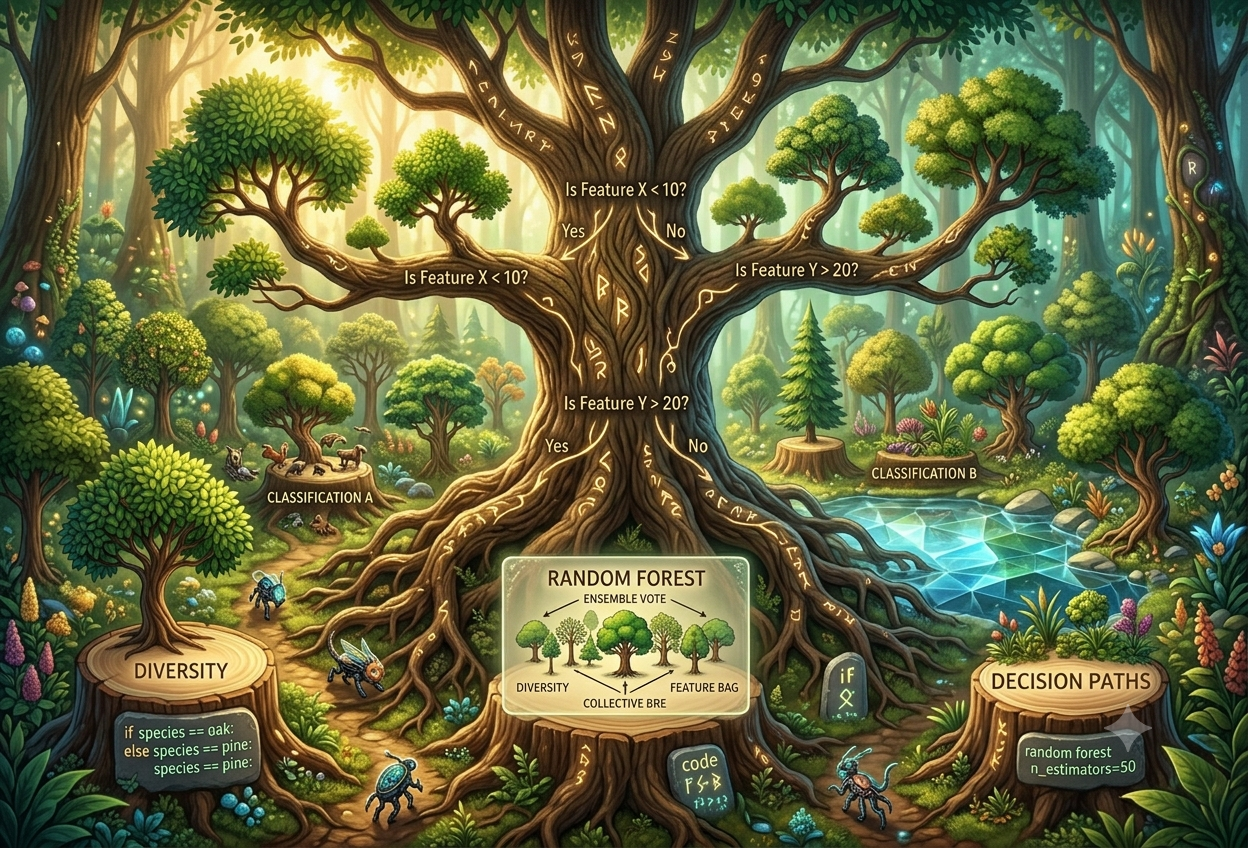
Decision Trees & Random Forests
What Is a Decision Tree?
Picture the game “20 Questions.” Someone is thinking of an animal, and you have to guess it by asking yes-or-no questions: “Does it have fur?” “Does it live in water?” “Is it bigger than a dog?” Each answer narrows things down until you land on a confident guess. A decision tree is a computer program that plays exactly this game with data.
“In a decision tree, each internal node represents a test on an attribute, each branch represents the outcome of that test, and each leaf node represents a final decision.”— Standard Definition, Machine Learning Literature
A decision tree is a supervised machine learning algorithm — meaning it learns from examples that already have known, correct answers — and it can be used for two main jobs: classification (sorting things into categories, like “spam” or “not spam”) and regression (predicting a number, like a house price). It gets its name because, when you draw it out, it looks like an upside-down tree: a single trunk at the top that splits into branches, which split again into smaller branches, until they end in leaves.
Every decision tree is built from three kinds of parts. The root node sits at the very top and represents the entire dataset before any questions have been asked. Decision nodes (sometimes called internal nodes) are the points where the tree asks a question about one feature of the data — such as “Is income above ₹50,000?” — and splits into two or more branches depending on the answer. Leaf nodes sit at the very ends of the branches and hold the tree’s final answer: a category label for classification, or a number for regression.
Imagine you are sorting your toy box. You might first ask, “Is it soft?” If yes, it goes in the stuffed-animal pile. If no, you ask another question: “Does it have wheels?” If yes, cars pile. If no, blocks pile. You just built a decision tree in your head! Each question you ask is like a branch, and each pile you end up with is like a leaf.
What makes decision trees special is that a computer does not just guess questions randomly — it mathematically figures out which question, asked at each step, does the best job of separating the data into clean, organised groups. We will explore exactly how it picks those questions in the next section.
Why Decision Trees Matter
Decision trees became one of the most widely taught algorithms in machine learning because they mirror how humans actually reason. Doctors diagnose patients by asking a sequence of questions. Banks decide on loans by checking a series of conditions. Decision trees simply formalise that step-by-step questioning into a structure a computer can learn automatically from data, rather than a human having to write out every rule by hand.
Used to help flag whether a patient’s symptoms point toward a particular condition, based on test results and history.
DiagnosisHelps decide whether to approve a loan or flag a transaction as suspicious, based on income, history, and behaviour.
FinancePredicts whether a shopper is likely to buy a product, based on browsing habits and past purchases.
E-CommerceHow a Tree Thinks: Splitting Rules
A decision tree could ask hundreds of possible questions about your data. So how does it pick the right one, in the right order? It uses a mathematical scorecard to measure how “messy” or how “clean” each possible split would make the resulting groups — and then it chooses whichever question cleans things up the most.
This idea of messiness has a formal name: impurity. A group of data is considered pure if every single item in it belongs to the same category — for example, a leaf containing only customers who bought a product. A group is impure if it is a jumbled mix of different categories. The tree’s whole strategy, at every single step, is to pick the question that reduces impurity by the largest possible amount.
Imagine a bag of marbles that is a mix of red and blue. That bag is “impure” — it’s mixed up. Now imagine you sort them into two bags: one with only red marbles and one with only blue marbles. Those bags are “pure” — nothing mixed in them. A decision tree always tries to sort its data into bags that are as pure as possible, one good question at a time.
Gini Impurity
The most commonly used impurity measure is called Gini impurity (used by default in many popular machine learning libraries). It calculates the probability that, if you picked two random items from a group, they would belong to different categories. A Gini score of 0 means the group is perfectly pure — every item belongs to the same class. A Gini score of 0.5 (for a two-category problem) means the group is as mixed up as it could possibly be, a true coin-flip of uncertainty.
Entropy & Information Gain
An alternative measure, entropy, is borrowed straight from information theory — the branch of mathematics that studies how much “surprise” or uncertainty is contained in a message. Entropy is 0 when a group is perfectly pure, and reaches its maximum value of 1 when a group is split exactly evenly between two categories. Whichever measure is used, the tree calculates a value called information gain: the improvement in purity achieved by splitting on a particular question, compared to leaving the data unsplit. The tree compares information gain across every possible question it could ask, and selects whichever one gives it the biggest improvement.
Gini vs. Entropy — Does It Matter Which One You Use?
In practice, Gini impurity and entropy almost always lead to very similar trees. The main practical difference is computational: Gini impurity only requires squaring probabilities, while entropy requires a logarithm calculation, which is slightly slower to compute. This is why Gini is the default choice in many libraries, especially when speed matters across large datasets or when building hundreds of trees inside a random forest. Entropy is sometimes preferred in academic or information-theory-oriented contexts, or when working with highly imbalanced classes, where its slightly different sensitivity to rare categories can occasionally produce a marginally better split.
| Measure | Pure Score | Most Impure Score | Computation | Common Use |
|---|---|---|---|---|
| Gini Impurity | 0 | 0.5 (binary case) | Faster — no logarithms | Default in most libraries; used in CART, Random Forests |
| Entropy | 0 | 1.0 (binary case) | Slower — uses logarithms | Information-theory contexts; ID3, C4.5 algorithms |
A decision tree never “guesses.” At every single branching point, it mathematically tests every possible question it could ask about every feature, measures how much each question would reduce impurity, and picks the single best one. This repeats over and over, branch after branch, until the tree decides it is time to stop.
Building a Tree, Step by Step
Now that we know how a tree picks its questions, let’s walk through the complete journey a decision tree takes — from a pile of raw, unsorted data, all the way to a finished, working model ready to make predictions.
This process is called recursive partitioning, and it works top-down. The algorithm begins with the entire dataset at the root, searches across every feature and every possible threshold for splitting that feature (for example, every possible age cutoff), and selects the single split that produces the purest possible child groups. It then treats each of those child groups as its own smaller problem, and repeats the exact same search inside each one — branching further and further down, like a tree growing new limbs.
When Does the Tree Stop Growing?
Left completely unchecked, a tree could keep splitting until every single leaf contains just one data point — which sounds accurate, but is actually a serious problem (we will cover exactly why in Section 05). To prevent this, the tree-building process is told to stop branching once it hits any of several conditions:
- Maximum depth reached: A limit is set on how many levels of questions the tree is allowed to ask before it must stop and produce a final leaf.
- Minimum samples per leaf: The tree is told not to create a leaf with fewer than a certain number of data points in it, to avoid leaves based on just one or two unusual examples.
- No further improvement: If no remaining split would meaningfully reduce impurity any further, the branch stops growing there.
- Perfect purity achieved: If every data point remaining in a group already belongs to the same class, there is nothing left to split — that branch is finished.
Pruning: Trimming Back an Overgrown Tree
Sometimes a tree is allowed to grow fully first, and then it gets trimmed back afterward — a process called pruning, named after the gardening technique of cutting back overgrown branches. In pruning, branches that add complexity without meaningfully improving the tree’s accuracy on new, unseen data are removed. This is typically done by holding back a separate slice of data (called a validation set) that the tree never used for training, building the full tree, and then snipping away branches one at a time, checking each time whether accuracy on the validation set gets better, worse, or stays the same.
Imagine studying for a test by memorising the exact answers to last year’s practice questions, word for word — including the typos. You would do perfectly on that old practice test, but terribly on the real exam, because you memorised instead of actually learning the topic. Pruning is like a teacher saying, “Don’t memorise every tiny detail — just learn the general rule,” so the tree can handle new questions it has never seen.
Classification vs. Regression Trees
Decision trees come in two main flavours, depending on what kind of question they are trying to answer. Together, these two types are sometimes grouped under one umbrella name: CART, short for Classification And Regression Trees.
Predicts a category or label — answering questions with a fixed set of possible outcomes, like “Will this customer churn? Yes or No,” or “Is this email spam or not spam?” Each leaf holds a class label.
Predicts a continuous number — answering questions like “What will this house sell for?” or “How many units will sell next month?” Each leaf holds a numeric value, usually the average of the training examples that landed there.
The core splitting process described in Sections 02 and 03 works almost identically for both types — the tree is still searching for the question that best separates the data. The only real difference is in how “purity” gets measured. A classification tree measures purity using Gini impurity or entropy, since it cares about how mixed up the category labels are inside a group. A regression tree instead measures purity using something like variance, or the squared difference between each data point’s value and the average value in that group — because here, “pure” means all the numbers in the group are close together, not spread far apart.
A classification tree is like sorting your trading cards into types: “Fire,” “Water,” or “Grass.” A regression tree is more like guessing a number, such as how many marbles are in a jar, based on clues like the jar’s size and how heavy it feels. One sorts things into named groups; the other guesses a number.
A Worked Example
Imagine a small classification tree trying to predict whether a customer will buy a product, using three features: age, income, and whether they have purchased before. The tree might first split on “previous purchase,” since that single question turns out to separate buyers from non-buyers most cleanly. Within the “no previous purchase” branch, it might then split further on income, since income turns out to be the next most useful question for that remaining group. This process continues, branch by branch, until the stopping rules from Section 03 kick in and the leaves are finalised.
“A decision tree breaks a problem into a series of questions. Each question helps reduce uncertainty until the answer becomes clear.”
— Common Framing in Machine Learning EducationMulti-Class Problems
Classification trees are not limited to simple yes-or-no answers. A leaf can represent any one of several possible categories — for example, classifying a flower into one of three species based on petal measurements, or classifying a movie review as positive, negative, or neutral. The splitting logic stays exactly the same; the only change is that impurity is now calculated across three or more categories instead of two.
Strengths & Weaknesses of One Tree
Decision trees are loved for being easy to understand — but that simplicity comes with real trade-offs. Before we build up to random forests, it is worth pausing to honestly examine where a single decision tree shines, and where it tends to stumble.
✓ Strengths
- Extremely easy to interpret — you can trace the exact path from root to leaf and explain precisely why a prediction was made.
- Requires very little data preparation — handles both numeric and categorical features without needing to rescale anything.
- Naturally captures non-linear, complex patterns without any special feature engineering.
- Fast to train and fast to use for predictions, even on modest hardware.
- Mirrors human-style reasoning, which makes it ideal for regulated fields like finance and healthcare where decisions must be explainable.
✗ Weaknesses
- Prone to overfitting — a deep tree can end up memorising the noise and quirks of the training data instead of the real underlying pattern.
- Highly unstable — a tiny change in the training data, even a handful of different examples, can result in a completely different tree being built.
- Tends to favour features with many possible split points, which can sometimes distort which feature looks “important.”
- Struggles to express certain simple relationships (like a diagonal boundary) efficiently, since it can only ask one feature at a time, splitting the data into rectangular regions.
- A single tree’s accuracy on new, unseen data is usually lower than more advanced approaches.
Overfitting, Explained Properly
Overfitting happens when a model becomes so finely tuned to its training data that it loses the ability to generalise to new examples. In a decision tree, this typically shows up as a very deep tree with many tiny leaves, each one built around just a handful of unusual training examples rather than a genuinely useful pattern. The tree gets excellent — sometimes perfect — accuracy on the data it was trained on, but performs poorly the moment it sees fresh, real-world data.
Imagine memorising the answers to last week’s spelling test instead of actually learning to spell. You’d ace that exact test again, but fail a new one with different words. That’s overfitting — getting really good at the exact examples you practiced on, without actually learning the general skill.
Instability, Explained Properly
The second major weakness — instability — means that decision trees are very sensitive to small changes in their training data. Because each split depends entirely on the split before it, changing or removing even a small number of training examples can cause the tree to choose a completely different question at the root, which then cascades into an entirely different shape for the rest of the tree. This sensitivity is technically called high variance, and it is the single biggest motivation behind the next big idea in this guide: instead of relying on one tree’s opinion, why not ask a whole crowd of trees and combine their answers?
From One Tree to a Forest
If a single decision tree can be unstable and prone to memorising noise, what if instead of trusting just one tree’s opinion, you asked hundreds of slightly different trees and let them vote? That simple but powerful idea is exactly what a random forest does.
Imagine you are choosing a holiday destination, so you ask one well-travelled friend for advice. They give you a recommendation based on their own past trips, likes, and biases. Now imagine instead you ask fifty different friends, each with different travel experiences and tastes, and you go with whichever destination gets recommended by the most people. That second approach — combining many independent opinions — is far less likely to be thrown off by any single friend’s unusual preference. This is the “wisdom of the crowd,” and it’s the entire foundation of a random forest.
This general strategy — building many models and combining their predictions — is called ensemble learning. A random forest is one of the most popular and effective ensemble methods, and it is built specifically out of many decision trees. The key insight is that while any one tree might make mistakes due to overfitting or instability, those mistakes tend to be somewhat random and different from tree to tree. When you average together (for regression) or vote across (for classification) the predictions of many such trees, the individual errors tend to cancel each other out, while the genuine underlying pattern — which most trees pick up on — gets reinforced.
Imagine your whole class guessing how many candies are in a jar. Some guesses will be too high, some too low — but if you average every single guess in the class together, that average is usually much closer to the real number than almost any one person’s individual guess. A random forest works the same way: lots of “guesses” (trees) combined together beat any single guess on its own.
But Wait — Won’t All the Trees Just Be the Same?
This is the crucial question, and the answer is the real engineering trick behind random forests: if you simply built the same decision tree on the exact same data a hundred times, you would get a hundred identical trees, and averaging them would achieve absolutely nothing. For the “wisdom of the crowd” effect to work, each tree in the forest needs to be meaningfully different from the others — different enough that their mistakes don’t all point in the same direction. Random forests achieve this difference through two clever sources of randomness, which we explore in full in the next section: each tree sees a different random sample of the data, and each tree is restricted to a different random subset of features when deciding how to split.
The idea of combining multiple models through a technique called bootstrap aggregating, or “bagging,” was introduced by statistician Leo Breiman in the mid-1990s. Breiman later extended this idea specifically to decision trees, adding the second layer of feature-level randomness, and formally introduced what we now call the “random forest” algorithm in a landmark 2001 paper. It remains, decades later, one of the most reliable, widely-used algorithms in practical machine learning — frequently chosen as a strong first attempt before reaching for more complex models.
How Random Forest Works
Let’s open up the engine and look at exactly what happens when a random forest is built — from raw data, to a hundred slightly different trees, to one final combined prediction.
Step 1 — Bootstrap Sampling (Bagging)
For each tree the forest is going to build, it first creates a new training set by randomly sampling from the original data with replacement — meaning the same data point can be picked more than once, and some data points might not get picked at all. This technique is called bootstrap sampling, and the overall strategy of training many models on different bootstrap samples and combining them is called bagging (short for “bootstrap aggregating”). On average, each bootstrap sample ends up containing roughly two-thirds of the unique data points from the original dataset, each tree therefore “sees” a slightly different slice of reality.
Step 2 — Random Feature Selection
This is the second, and arguably more important, source of randomness. When a normal decision tree looks for the best split at a node, it considers every available feature. A tree inside a random forest, by contrast, is only allowed to consider a small random subset of the available features at each split. This forces different trees to discover different, sometimes less-obvious patterns in the data, since the single most powerful feature in the whole dataset will not even be available as an option in many of the splits across many of the trees.
Step 3 — Grow Each Tree
Using its own bootstrap sample and its own restricted choice of features at every split, each tree grows using exactly the same splitting logic described in Sections 02 and 03 — repeatedly choosing the split with the highest information gain, branch after branch, until a stopping condition is reached. Random forest trees are often allowed to grow quite deep and are not pruned the way a standalone tree might be, because the averaging step that follows naturally corrects for any individual tree’s overfitting.
Step 4 — Combine the Predictions
Once every tree in the forest has been grown, a brand-new data point is run through all of them simultaneously. For a classification task, each tree casts one “vote” for whichever category it predicts, and the forest’s final answer is whichever category received the most votes — a process called majority voting. For a regression task, each tree outputs a number, and the forest’s final answer is simply the average of all those numbers.
The Out-of-Bag (OOB) Bonus
Because each tree’s bootstrap sample leaves out roughly a third of the original data, that leftover data — called the out-of-bag (OOB) data — can be used as a free built-in test set for that particular tree. By checking how well each tree predicts the data it never saw during its own training, random forests can estimate their overall accuracy without needing to set aside a separate validation set at all, which is a particularly handy efficiency when data is limited.
Imagine your teacher splits your class into small study groups, but gives each group a slightly different mix of practice questions to study from — some questions overlap between groups, some don’t. Then, for a pop quiz, each group answers using only what they personally studied. Since each group studied something a little different, the questions one group might get wrong, another group studying different material would likely get right — and when you combine everyone’s best answers, the overall class score ends up better than almost any single group could have managed alone.
Feature Importance — A Useful Side Effect
Because a random forest tracks how much each feature contributes to reducing impurity across every split, in every tree, it can automatically rank which features mattered most to its predictions overall — a property called feature importance. This is extremely useful in practice: a data scientist can train a random forest, look at its feature importance scores, and learn which variables actually drive the outcome being predicted, even before building a final, more carefully tuned model.
Tuning Knobs & Hyperparameters
Both decision trees and random forests come with adjustable settings — called hyperparameters — that a practitioner chooses before training begins. Getting these right is often the difference between a model that performs adequately and one that performs excellently.
Think of hyperparameters like the settings on a video game’s difficulty menu. You choose them before you start playing, and they shape how the whole game behaves. A decision tree or random forest has similar settings you choose before training begins, and they shape how the model learns.
Tree-Level Settings
Caps how many levels of questions a tree is allowed to ask. Smaller values reduce overfitting but may miss complex patterns.
Sets the minimum number of data points required in a leaf. Higher values produce smoother, less overfit trees.
The minimum number of samples a node must have before the tree is even allowed to consider splitting it further.
Forest-Level Settings
The number of trees in the forest. More trees generally improve stability and accuracy, but increase training time and memory use.
Most ImportantHow many features each tree is allowed to randomly consider at every split. Lower values increase diversity between trees.
How many processor cores can be used to train trees simultaneously. Setting this to use all available cores speeds up training significantly.
A fixed “seed” number that makes the randomness reproducible — useful so the exact same forest can be rebuilt later for testing or comparison.
The n_estimators Trade-off
The number of trees is usually the single most impactful setting in a random forest. As more trees are added, predictions tend to become steadily more accurate and more stable, since the averaging effect described in Section 06 strengthens with a larger crowd. However, this improvement has diminishing returns — going from 10 trees to 100 trees usually helps a great deal, while going from 500 to 1,000 trees often barely moves the needle, while still doubling the time and memory required.
A very common and effective starting strategy is to begin with a moderate number of trees (such as 100), use the default settings for everything else, and only fine-tune further if the model’s accuracy genuinely demands it. Random forests are famous for performing reasonably well even with their default settings, which is part of why they remain such a popular first choice for new machine learning problems.
Decision Tree vs. Random Forest
With both algorithms now explained in full, let’s put them directly side by side. Neither one is universally “better” — each is the right tool for a different situation.
| Property | Decision Tree | Random Forest |
|---|---|---|
| Structure | A single tree | An ensemble of many trees |
| Interpretability | Very high — easy to trace and explain | Lower — harder to explain a single combined decision |
| Overfitting Risk | High, especially with deep trees | Much lower, thanks to averaging across trees |
| Stability | Sensitive to small data changes | Much more stable and consistent |
| Training Speed | Fast — only one tree to build | Slower — many trees must be built |
| Prediction Speed | Fast — a single pass through one tree | Slower — every tree must be consulted and combined |
| Accuracy (typical) | Good on simple problems | Usually higher, especially on complex data |
| Handling Outliers | More sensitive to unusual data points | More robust, thanks to averaging |
| Feature Importance | Available, but less reliable | Available and generally more trustworthy |
| Best Dataset Size | Works on both small and large datasets | Shines especially on larger, more complex datasets |
When Should You Reach for a Decision Tree?
- When you need a model that a non-technical stakeholder can look at and understand, branch by branch.
- When you are working with a small dataset and training speed or simplicity matters more than squeezing out every last percentage point of accuracy.
- When regulatory or compliance requirements demand a fully transparent, auditable decision-making process — common in lending and insurance.
- When you simply want a fast first look at which features in your data seem to matter, before investing in a heavier model.
When Should You Reach for a Random Forest?
- When predictive accuracy and robustness matter more than being able to fully explain every single decision.
- When your dataset is large, complex, or contains noisy or messy real-world data with outliers.
- When you suspect overfitting will be a problem with a single tree and want a built-in safeguard against it.
- When you want a strong, reliable “default” model to benchmark against before trying more advanced techniques.
“Use a decision tree when interpretability is paramount. Use a random forest when accuracy and robustness matter more than explainability.”
— Common Guidance in Applied Machine LearningWhere They Work in the Real World
Decision trees and random forests are not just classroom exercises — they quietly power decisions behind the scenes across some of the largest industries in the world, often without people realising it.
Banking & Finance
Banks use random forests to evaluate credit risk, learning from thousands of historical loan applications which patterns are associated with successful repayment versus default, then applying that learning to new applicants. The natural diversity across many trees helps the model avoid being fooled by a handful of unusual cases or biases hiding in the data.
Fraud Detection
Credit card companies face an extremely lopsided problem: fraudulent transactions might make up only a tiny fraction of a percent of all transactions. Random forests are particularly well-suited to this kind of imbalanced data, flagging unusual behaviour — like a sudden purchase in a foreign country — in real time.
Healthcare & Medicine
Hospitals use random forests to help predict patient readmission risk or flag early warning signs of conditions such as diabetes or heart disease, by analysing combinations of symptoms, lab results, medical history, and demographic information.
Trading & Markets
Investment platforms use random forests to study patterns across technical indicators, trading volumes, and market sentiment, helping traders identify potentially useful signals — though, as with all market prediction, no model removes the underlying unpredictability of markets.
E-Commerce
Online retailers use these models to predict whether a shopper is likely to enjoy or purchase a particular product, and to flag suspicious-looking transactions for review before they are processed.
Spam & Content Filtering
Email providers and content platforms use tree-based models as part of their systems for distinguishing spam from genuine messages, by learning the patterns that separate the two over millions of examples.
Every time your bank decides whether to approve your parents’ loan, every time your favourite shopping app suggests something you might like, or every time your email automatically sorts out spam — there’s a good chance a decision tree or a random forest of trees is quietly working behind the scenes, learning from thousands of past examples to make that call.
Why These Algorithms Are So Widely Trusted
Part of the reason decision trees and random forests remain so popular across industries — even decades after they were first introduced — is that they require comparatively little data preparation, can be trained reasonably quickly, work well on both numeric and categorical data, and (in the case of random forests especially) tend to produce reliably strong results even before careful tuning. In regulated industries like banking and healthcare, the relative explainability of decision trees also gives them a real practical edge over more opaque “black box” models.
Pros, Cons & When to Use Which
Having looked at decision trees in detail back in Section 05, let’s now give random forests the same honest treatment — because no algorithm, no matter how popular, is a perfect fit for every problem.
✓ Random Forest Strengths
- Significantly reduces overfitting compared to a single decision tree, thanks to averaging across many diverse trees.
- Handles large datasets with many features without losing accuracy or slowing down dramatically.
- Works well for both classification and regression problems, using the same underlying mechanism.
- Robust to outliers and noisy data, since unusual data points only influence a portion of the trees.
- Provides genuinely useful feature importance scores, helping practitioners understand their data.
- Performs reasonably well even with default hyperparameter settings — a great “first model” choice.
✗ Random Forest Limitations
- Much harder to interpret than a single tree — you cannot easily trace “the one path” that led to a decision.
- More computationally expensive, especially with a very large number of trees, since training and prediction time grow accordingly.
- It is a predictive tool, not a descriptive one — it is built to make accurate guesses, not to clearly explain the relationships between variables the way simpler statistical models can.
- Slower to generate predictions once trained, compared to a single tree, since every individual tree must be consulted and combined.
- Most popular implementations still require some preprocessing for missing values, even though the algorithm is broadly tolerant of messy data otherwise.
A random forest is amazing at giving you the right answer, but it’s not great at explaining exactly why — sort of like asking your entire class for the answer to a hard maths problem and getting the most popular answer, without each individual student showing all their working.
The Explainability Trade-off
This tension between accuracy and explainability comes up constantly in real machine learning work, and it’s worth understanding clearly. A single decision tree gives a transparent answer that is easy to justify to a regulator, a customer, or a colleague — but it is more likely to be wrong, especially on complex or noisy data. A random forest is typically more accurate and more reliable — but its final answer comes from combining the votes of potentially hundreds of trees, making it much harder to produce a simple, human-readable explanation for any individual prediction. Specialised techniques exist to help bridge this gap (such as analysing feature importance, or more advanced explanation methods used in modern machine learning), but they add extra complexity on top of the model itself.
If you genuinely need to explain each individual prediction in plain language — to a regulator, an auditor, or a worried customer — lean toward a decision tree, possibly pruned to stay small and readable. If your priority is the most accurate and dependable prediction possible, and explainability is a secondary concern, lean toward a random forest.
Beyond Random Forest
Random forests are a brilliant evolution of the basic decision tree, but they are not the final word in tree-based machine learning. Understanding what comes after them helps put the whole family of algorithms in perspective.
Random forests build all of their trees independently and in parallel — every tree is grown separately, without paying attention to what the other trees got right or wrong, and the results are combined only at the very end through voting or averaging. This general family of methods is called bagging. A different family of ensemble methods, called boosting, takes a fundamentally different approach: it builds trees one after another, in sequence, where each new tree is specifically trained to focus on correcting the mistakes made by the trees that came before it.
CART Introduced
Classification and Regression Trees are formalised, laying the mathematical groundwork for modern decision trees.
Bagging
Leo Breiman introduces bootstrap aggregating, the statistical foundation that random forests are built on.
Random Forest
Breiman formally combines bagging with random feature selection, creating the random forest algorithm.
Gradient Boosting
Boosting methods mature, building trees sequentially so each new tree corrects the previous trees’ errors.
XGBoost & Modern Boosted Trees
Highly optimised gradient boosting libraries become dominant in machine learning competitions and industry applications, prized for their accuracy.
Bagging vs. Boosting, in Plain Language
Many trees grown independently and in parallel, each on a random slice of data and features, then combined by vote or average. Mainly fights overfitting and instability.
Trees grown one after another in sequence, with each new tree focused on fixing the previous trees’ mistakes. Mainly fights underfitting, often squeezing out higher accuracy.
Bagging is like asking fifty friends the same question all at once, separately, then going with the most popular answer. Boosting is more like asking one friend, seeing where they got it wrong, then asking a second friend who specifically tries to fix that mistake, then a third friend who fixes whatever is still wrong, and so on — each new friend building on the last one’s lessons.
Boosting methods, especially modern, highly engineered libraries, frequently achieve even higher accuracy than random forests on many problems, which is part of why they dominate machine learning competitions today. However, they also tend to be more sensitive to their hyperparameters, slower to tune correctly, and somewhat more prone to overfitting if not handled carefully — trade-offs that make random forests an excellent, more forgiving starting point before reaching for boosting.
Common Mistakes & Best Practices
To close out this guide, here are the practical lessons that separate a working decision tree or random forest model from one quietly undermined by avoidable mistakes.
Common Mistakes
- Letting a single tree grow unchecked: Forgetting to set a maximum depth or minimum leaf size is one of the fastest ways to produce a badly overfit decision tree.
- Evaluating only on training data: A model that looks perfect on the data it was trained on can still fail badly on new data — always test on data the model has never seen.
- Ignoring class imbalance: If one category vastly outnumbers another (as in fraud detection), a model can achieve high accuracy just by always guessing the majority class — accuracy alone can be a misleading metric in these situations.
- Using too few trees in a forest: A random forest with only a handful of trees loses much of the stability benefit that makes the whole approach worthwhile.
- Misreading feature importance as causation: A feature being “important” to a model’s predictions does not necessarily mean it causes the outcome — correlation and causation remain different things.
- Not handling missing data: Most popular implementations of these algorithms still expect missing values to be addressed beforehand, despite the algorithms otherwise tolerating messy data well.
Best Practices
- Always split your data into separate training and testing sets, so you can honestly measure how well the model generalises.
- Start with sensible default hyperparameters, then tune gradually — random forests in particular perform well even without heavy tuning.
- Use cross-validation, where the data is split multiple different ways and results are averaged, for a more reliable measure of true performance.
- Examine feature importance scores to sanity-check that the model is learning from genuinely meaningful signals, not data quirks.
- For high-stakes decisions affecting real people — loans, medical diagnoses, hiring — pair model accuracy with genuine efforts toward explainability and human oversight.
- When facing imbalanced classes, look beyond plain accuracy to metrics like precision, recall, or the out-of-bag error estimate described in Section 07.
It’s a bit like studying for a test: don’t just memorise the practice questions word-for-word (that’s overfitting), make sure you actually test yourself on new, different questions before the real exam (that’s testing on unseen data), and if almost every practice question has the same easy answer, don’t assume the real test will be that easy too (that’s class imbalance).
A decision tree is, at its heart, a simple and intuitive idea: ask the most useful question you can at every step, and keep narrowing things down until you reach an answer. A random forest takes that same simple idea and multiplies it — building many slightly different trees, each seeing a different slice of the data and a different subset of features, and combining their collective judgement into one far more accurate and dependable prediction. Together, these two algorithms remain, decades after their invention, some of the most trusted, widely deployed tools in the entire field of machine learning — proof that sometimes the most powerful ideas in AI are also the easiest to explain to a 10-year-old.
Sources & References
Direct comparison covering interpretability, overfitting, training time, and stability between the two algorithms.
Technical walkthrough of tree construction, splitting logic, and ensemble aggregation.
Classification-focused explainer with practical framing for beginners.
Step-by-step tutorial covering core mechanics and use cases.
Industry-oriented overview of where these algorithms are applied in business contexts.
Concise breakdown of the practical differences and when to choose each algorithm.
Broad guide covering theory, math, and worked examples.
Detailed coverage of how random forest works, hyperparameters, advantages, and limitations.
Educational overview aimed at learners new to ensemble methods.
Hands-on notebook-style explainer with beginner-friendly framing and worked code examples.
In-depth guide covering bagging, hyperparameters, feature importance, and real-world applications.
Comparative exploration spanning single trees through to modern boosting methods.
Interview-prep-oriented explainer covering core concepts and common questions.