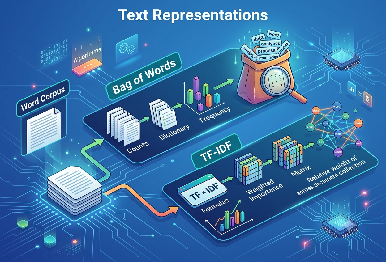
Text Representations
Bag of Words
& TF-IDF
Every day, billions of messages, emails, reviews and articles are written by humans. Computers can store those words — but can they truly understand them? This guide explores Bag of Words and TF-IDF, the two foundational ideas that taught machines how to read.
Every day, billions of messages, emails, reviews, and articles are written by humans. Computers can store those words — but can they truly understand them? This guide explains the first clever tricks scientists invented to teach computers how to read.
Imagine you have a robot friend who is very good at maths but has never seen a book before. You hand it a story and ask, “Is this story about cats or dogs?” The robot stares blankly — it only speaks numbers, not words! So how do we translate human language into a form computers can work with? That is precisely the puzzle that Natural Language Processing (NLP) tries to solve.
Over many decades, clever researchers came up with two foundational ideas — Bag of Words (BoW) and Term Frequency–Inverse Document Frequency (TF-IDF) — that turned paragraphs of human text into neat tables of numbers that computers could finally start to understand and compare.
Think of it like sorting your LEGO bricks into buckets. You don’t care about the order you throw them in — you just want to know: how many red bricks? How many blue bricks? Bag of Words does something very similar with words in a sentence!
All of that data above is mostly text. Without methods like BoW and TF-IDF, none of it could be processed by machine learning algorithms. These two techniques form the very alphabet of modern AI’s ability to deal with language.
Computers are fluent in numbers. Language is full of meaning, emotion, sarcasm, and context. Bridging that gap is one of the biggest challenges in Artificial Intelligence.
When you look at the word “bank”, you instantly know from context whether it means the side of a river or a place to keep money. A computer, looking at just the raw letters B-A-N-K, has no idea which meaning applies. This is called the ambiguity problem, and it is just one of many challenges in language.
Why Can’t Computers Just Read Words?
All computers do internally is add and multiply numbers. They cannot natively process the letter “A” — only its numeric code (65 in ASCII). Machine learning models need purely numeric input.
The English language alone has over 170,000 words in active use. New words are invented constantly (think “selfie” or “meme”). Any text conversion system must handle this enormous variety.
“Dog bites man” and “Man bites dog” contain the same words but mean very different things. Some tasks need word order; others do not. Choosing the right representation matters.
“Oh great, another Monday!” The word “great” is positive, but the whole sentence is negative. Computers struggle with these hidden layers of human expression.
The journey to solve these problems started with the simplest possible approach: what if we just count words? That idea gave birth to the Bag of Words model — humble in design, yet surprisingly powerful in practice.
FIG 01 — The pipeline: from raw human text to numeric vectors that machine learning models can consume.
Imagine emptying every word from a sentence into a cloth bag and shaking it around. You lose track of the order, but you can still count how many times each word appears. That is the essence of the Bag of Words model.
The Bag of Words approach was one of the earliest and most intuitive ways scientists tried to represent text for computers. The core idea is beautifully simple: treat each piece of text (called a document) as just a collection of words, completely ignoring the sequence in which those words appear. What matters is not where a word is but how often it shows up.
A Bag of Words is a text representation method that converts a document into a numerical vector by counting how many times each word from a fixed vocabulary appears — without caring about word order or grammar.— NLP Fundamentals, Text Representation Methods
Step-by-Step: How BoW Works
Let’s walk through a real example together. Say we have three short sentences:
Sentence A: “The cat sat on the mat”
Sentence B: “The cat sat on the hat”
Sentence C: “The dog sat on the mat”
Step 1 — Build a Vocabulary
Collect every unique word that appears across all your documents. This is called the vocabulary or corpus vocabulary. In our case 7 unique words make up the entire vocabulary: the, cat, sat, on, mat, hat, dog.
Step 2 — Count Each Word Per Document
For every sentence, go through the vocabulary and write down how many times each word appears. If a word doesn’t appear, write 0.
| Document | the | cat | sat | on | mat | hat | dog |
|---|---|---|---|---|---|---|---|
| Sentence A | 2 | 1 | 1 | 1 | 1 | 0 | 0 |
| Sentence B | 2 | 1 | 1 | 1 | 0 | 1 | 0 |
| Sentence C | 2 | 0 | 1 | 1 | 1 | 0 | 1 |
Each row in the table above is called a vector — a list of numbers that represents one document. Sentence A is now the vector [2, 1, 1, 1, 1, 0, 0]. This is something a computer can work with!
Step 3 — Use the Vectors
Now that every document is a row of numbers, we can do all sorts of clever maths — like measuring how similar two documents are by checking how close their vectors are to each other in mathematical space.
FIG 02 — Bag of Words converts a sentence into a count vector; similar documents end up close together in vector space.
Imagine a recipe card. Instead of following the instructions step by step, you dump all the ingredients on the table and count them: 2 eggs, 1 cup of flour, 3 spoons of sugar. You lost the cooking order, but you know what is in the recipe — and that’s often enough to guess what food it is!
BoW is a great starting point, but it has some significant blind spots. Understanding what it gets wrong is just as important as knowing what it gets right.
Problem 1 — Common Words Dominate
Words like “the”, “a”, “is”, and “and” appear in almost every sentence in the English language. In a BoW model, these high-frequency words get very large counts — making them look extremely “important” when in reality they carry almost no meaning about the topic. These are called stop words.
Problem 2 — Order Is Completely Lost
Consider these two sentences:
- “The dog bit the man” — A dog attacked a human. Sad but not unusual.
- “The man bit the dog” — A human attacked a dog. Very unusual headline news!
In a BoW model, both sentences produce identical vectors. The counts of “the”, “dog”, “bit”, “man” are the same. The computer cannot tell these sentences apart — a huge problem for tasks needing real understanding.
Problem 3 — Huge and Sparse Vectors
Real-world vocabularies can have hundreds of thousands of words. If you are working with a collection of news articles, your vocabulary might contain 80,000 words. Every document then becomes a vector with 80,000 numbers — and most of those numbers will be zero (since any single article uses only a small fraction of all words). This is called sparsity, and it wastes a huge amount of computer memory and slows down processing.
Problem 4 — No Sense of Word Importance
Here is the biggest problem of all: BoW treats every word equally. The word “the” and the word “photosynthesis” both count as one occurrence each — yet clearly “photosynthesis” is far more informative about the topic of a biology article than “the” ever could be. BoW has no way to express that some words are more meaningful than others.
Scientists noticed that words appearing in almost every document are not very useful for distinguishing between topics. But words that appear a lot in one document but rarely elsewhere? Those are the meaningful ones. That observation became the core idea of TF-IDF.
TF-IDF doesn’t just count words — it measures how important a word is to a specific document compared to all other documents. It rewards rare, meaningful words and punishes common, useless ones.
TF-IDF stands for Term Frequency – Inverse Document Frequency. It was developed by computer scientist Karen Spärck Jones in 1972 and remains one of the most widely used text analysis tools in the world today. The technique elegantly combines two separate measurements into a single importance score.
Karen Spärck Jones Invents IDF
British computer scientist Karen Spärck Jones publishes the concept of inverse document frequency, which would later be combined with term frequency to form TF-IDF. Her work was groundbreaking and is only now receiving the recognition it deserves.
Salton & Buckley Formalise TF-IDF
Gerard Salton and Christopher Buckley publish a comprehensive paper formalising TF-IDF weighting in information retrieval systems, giving it the form we recognise today.
Search Engines Adopt TF-IDF
Early web search engines — including early versions of Google’s ranking algorithms — incorporate TF-IDF as a core component for determining which documents are most relevant to a user’s query.
Still Widely Used
Despite the rise of deep learning, TF-IDF remains a competitive baseline for text classification, keyword extraction, and document retrieval — especially when training data is limited.
Part 1 — Term Frequency (TF)
The first component, Term Frequency, answers a simple question: “How often does this word appear in this particular document?”
If you have a 100-word document and the word “cat” appears 5 times, then the Term Frequency of “cat” in that document is 5 ÷ 100 = 0.05. Dividing by the total number of words is called normalisation — it ensures that a 1,000-word document doesn’t automatically get higher scores than a 100-word document just because it’s longer.
where t = the term (word) and d = the document
Part 2 — Inverse Document Frequency (IDF)
This is where TF-IDF gets clever. The second component, Inverse Document Frequency, asks: “In how many documents does this word appear at all?”
If a word appears in every single document in your collection, it’s probably not very helpful for identifying what makes any one document special — it’s likely a common word like “the” or “is”. But if a word appears in only 2 out of 1,000 documents, it must be doing something unique in those 2 documents — it’s probably a topic-specific, meaningful term.
The IDF formula takes the logarithm of how rare a word is across the whole collection. Using a logarithm prevents very rare words from getting wildly large scores, and keeps the numbers manageable.
where N = total number of documents, df(t) = number of documents containing term t
Imagine your school has 500 students. If 490 of them like pizza, saying “I like pizza” tells your friends nothing interesting about you — everyone likes pizza! But if only 3 students love fermented black beans, saying “I love fermented black beans” suddenly reveals something unique about you. IDF works the same way — it gives higher scores to words that are rare and distinctive.
Part 3 — Putting It Together: TF × IDF
The final TF-IDF score for any word in any document is simply the product of these two values:
high score = word appears often in this document but rarely elsewhere → very important
This scoring system naturally gives high scores to words that are both frequent in this document and rare across the collection — the hallmarks of a truly meaningful, topic-defining word. Common words like “the” or “and” have very low IDF scores (since they appear everywhere), so their TF-IDF score stays low no matter how often they appear in a single document.
FIG 03 — TF-IDF naturally filters out common, meaningless words and promotes rare, topic-specific terms.
Numbers make more sense when you see them in action. Let’s calculate TF-IDF scores for a real set of documents, step by step.
Doc 1: “The cat sat on the mat. The cat is fat.”
Doc 2: “The dog sat on the log. The dog likes to jog.”
Doc 3: “A cat and a dog are good friends.”
We will calculate the TF-IDF score for the word “cat” in Document 1.
Calculating Term Frequency (TF)
Document 1 has 10 words: the, cat, sat, on, the, mat, the, cat, is, fat. The word “cat” appears 2 times out of 10 total words.
cat appears 2 times in a 10-word document
Calculating Inverse Document Frequency (IDF)
We have 3 documents total (N = 3). How many documents contain the word “cat”? Doc 1 has it, Doc 3 has it — so 2 documents contain “cat” (df = 2).
3 total documents ÷ 2 documents containing “cat”
The Final TF-IDF Score
a modest score — “cat” is important but appears in more than one document
Now let’s compare scores for different words across our documents:
| Word | Doc | TF | IDF | TF-IDF Score | Interpretation |
|---|---|---|---|---|---|
| the | Doc 1 | 0.30 | 0.0 | 0.000 | Appears in every doc → useless |
| cat | Doc 1 | 0.20 | 0.176 | 0.035 | Appears in 2 of 3 docs → somewhat useful |
| fat | Doc 1 | 0.10 | 0.477 | 0.048 | Only in Doc 1 → distinctive! |
| jog | Doc 2 | 0.10 | 0.477 | 0.048 | Only in Doc 2 → very distinctive! |
| friends | Doc 3 | 0.125 | 0.477 | 0.060 | Only in Doc 3 → top scorer! |
Notice how “the” gets a score of exactly 0 because it appears in every document (so log(3/3) = log(1) = 0). Meanwhile, “fat”, “jog”, and “friends” — words unique to a single document — receive the highest scores. This is TF-IDF working exactly as intended!
“The word that matters most in a document is not the one that appears most often — it’s the one that appears often here but barely anywhere else.”
— The core insight behind TF-IDFBefore applying BoW or TF-IDF, raw text must go through a cleaning pipeline. Skipping this step leads to noisy, inaccurate results — like trying to count items in a messy room without first tidying it up.
Lowercasing
Without converting everything to lowercase, a computer would think “Cat” and “cat” are completely different words — which they clearly are not. Converting all text to lowercase ensures that identical words are counted as one, no matter how they were originally capitalised.
Removing Punctuation
Punctuation marks like commas, full stops, exclamation marks, and quotation marks carry no word meaning in BoW or TF-IDF. Removing them prevents “hello!” and “hello” from being counted as two separate vocabulary items.
Stop Word Removal
Stop words are ultra-common words — “the”, “a”, “an”, “is”, “in”, “on”, “of” — that appear so frequently they tell us nothing useful about what a document is about. Most NLP libraries (like NLTK or spaCy) include pre-built lists of stop words that you can remove in a single step.
Stemming & Lemmatisation
These two techniques reduce words to their base forms so that “running”, “runs”, and “ran” all count as the same word rather than three separate ones. This dramatically reduces vocabulary size and improves accuracy.
- Stemming is the cruder, faster method — it chops word endings off using rules, sometimes producing non-real words (e.g. “fishing” → “fish”, “studies” → “studi”).
- Lemmatisation is smarter and slower — it uses a dictionary to find the actual root form of a word (e.g. “better” → “good”, “are” → “be”).
Tokenisation
Finally, the cleaned text is split into individual tokens — usually individual words, but sometimes phrases or sub-words. This converts the text string into a list that the BoW or TF-IDF algorithm can iterate over.
Imagine you’re sorting a pile of coloured cards, but some cards say “RED”, some say “Red”, some say “red!”, and some say “reds”. Before you can count them properly, you need to: remove the “!” marks, make all letters the same case, and decide that “red” and “reds” are the same colour. That cleaning work is exactly what text preprocessing does!
Both BoW and TF-IDF are built right into the popular Python library scikit-learn. You can implement them in just a few lines of code.
Bag of Words with CountVectorizer
from sklearn.feature_extraction.text import CountVectorizer

# Our collection of documents
documents = [
    "The cat sat on the mat",
    "The cat sat on the hat",
    "The dog sat on the mat"
]

# Create the BoW model
vectorizer = CountVectorizer()
X = vectorizer.fit_transform(documents)

# See the vocabulary
print(vectorizer.vocabulary_)
# → {'cat': 0, 'dog': 1, 'hat': 2, 'mat': 3, 'on': 4, 'sat': 5, 'the': 6}

# See the count matrix
print(X.toarray())
# → [[1, 0, 0, 1, 1, 1, 2],   ← Sentence A
#     [1, 0, 1, 0, 1, 1, 2],   ← Sentence B
#     [0, 1, 0, 1, 1, 1, 2]]   ← Sentence C
TF-IDF with TfidfVectorizer
from sklearn.feature_extraction.text import TfidfVectorizer
import pandas as pd

documents = [
    "The cat sat on the mat",
    "The cat sat on the hat",
    "The dog sat on the mat"
]

# Create TF-IDF model (automatically removes stop words if asked)
tfidf = TfidfVectorizer(stop_words='english')
X_tfidf = tfidf.fit_transform(documents)

# Show as a readable dataframe
df = pd.DataFrame(
    X_tfidf.toarray(),
    columns=tfidf.get_feature_names_out(),
    index=['Sentence A', 'Sentence B', 'Sentence C']
)
print(df.round(3))
# Notice that "the", "on", "sat" disappear (stop words).
# Unique words like "dog", "hat", "cat" get the highest TF-IDF scores.
Finding the Most Important Keywords
import numpy as np

# Get the vocabulary list
feature_names = tfidf.get_feature_names_out()

# For each document, find the top 3 keywords by TF-IDF score
for i, row in enumerate(X_tfidf.toarray()):
    top_indices = np.argsort(row)[::-1][:3]
    top_keywords = [feature_names[j] for j in top_indices if row[j] > 0]
    print(f"Document {i+1} keywords: {top_keywords}")

# Output:
# Document 1 keywords: ['cat', 'mat']
# Document 2 keywords: ['hat', 'cat']
# Document 3 keywords: ['dog', 'mat']
Notice how the keywords extracted are meaningful and topic-specific — no stop words, no generic terms. This is TF-IDF doing its job.
Both methods convert text to numbers, but they do it differently and each has its own strengths and ideal use cases. Here is everything you need to know to choose between them.
| Feature | Bag of Words (BoW) | TF-IDF |
|---|---|---|
| Core Idea | Count how many times each word appears | Measure how important a word is to this document vs all documents |
| Word Order | Completely ignored | Completely ignored (same limitation) |
| Common Words | Given high counts (problematic) | Automatically down-weighted (very useful) |
| Output | Integer count vectors | Decimal weight vectors (0 to 1) |
| Complexity | Very simple to understand and implement | Slightly more complex but still straightforward |
| Best For | Simple classification, small datasets, teaching | Search engines, keyword extraction, larger datasets |
| Speed | Very fast | Fast (slightly slower due to IDF calculation) |
| Requires Large Corpus? | No | Better results with more documents |
Bag of Words — Pros & Cons
✓ STRENGTHS
- Incredibly simple to understand — even a child can grasp the counting idea
- Very fast to compute, even on huge datasets
- Works surprisingly well for simple tasks like spam filtering
- Perfect for getting started with NLP quickly
- No complicated parameters to tune
✗ WEAKNESSES
- Loses word order completely — sentences can’t be distinguished if they have the same words
- Treats all words equally regardless of their actual importance
- Common stop words inflate counts and add noise
- Vectors become enormous and mostly empty for large vocabularies
- No understanding of synonyms — “happy” and “joyful” are treated as unrelated
TF-IDF — Pros & Cons
✓ STRENGTHS
- Automatically recognises and down-weights common, unimportant words
- Produces much cleaner, more meaningful word importance scores
- Excellent for keyword extraction and document search
- Simple to use with scikit-learn in just 2-3 lines of code
- Still highly competitive against modern methods for many tasks
✗ WEAKNESSES
- Still loses word order — same limitation as BoW
- Does not understand word meaning or context
- New words not seen during training get zero scores
- The IDF calculation depends on the entire document collection
- Very rare words can get disproportionately high scores
BoW and TF-IDF are not just classroom exercises — they power real systems you interact with every day, from spam filters in your inbox to search bars on websites.
FIG 04 — BoW and TF-IDF power a wide range of real-world NLP applications across industries.
Search Engines
When you type a query into a search engine, TF-IDF has historically been used to rank which web pages are most relevant to your search. Pages where your search terms appear frequently but are rare across the web bubble up to the top. Even modern systems use TF-IDF-inspired components as part of their larger ranking pipelines.
Spam Detection
Email spam filters use BoW to identify patterns. Words like “FREE”, “WINNER”, “CLICK HERE”, and “LIMITED OFFER” appear very frequently in spam emails but rarely in genuine ones. A BoW model can learn these patterns and flag suspicious emails before they ever reach your inbox.
Sentiment Analysis
Companies use BoW and TF-IDF to analyse product reviews at massive scale. By training a model on thousands of labelled reviews (positive vs negative), the algorithm learns that words like “excellent”, “love”, and “amazing” predict positive reviews, while “broken”, “terrible”, and “waste” predict negative ones.
News Categorisation
News organisations need to automatically sort thousands of articles into categories like Sports, Finance, Technology, and Politics. TF-IDF extracts the most distinctive words from each article — words like “goal”, “transfer”, “midfielder” clearly signal Sports, while “revenue”, “quarterly”, “shares” signal Finance.
Plagiarism Detection
Universities use TF-IDF to compare student essays against a database of existing work. Two documents with very similar TF-IDF vectors — meaning they use the same unusual, topic-specific words in similar proportions — are likely to contain copied material and get flagged for further review.
Medical Record Analysis
Hospitals generate enormous amounts of clinical notes in free text. TF-IDF helps extract key symptoms, medications, and diagnoses from these notes, making it possible to search patient records, identify trends in disease, and assist doctors in finding relevant past cases quickly.
When you search for “funny cat videos” on YouTube, the site looks at all the video titles and descriptions. Videos that say “cat” and “funny” a lot, while those words are rare compared to all videos, show up first. That’s TF-IDF at work — the internet’s way of knowing what content best matches what you’re looking for!
BoW and TF-IDF were revolutionary when invented, but the field of NLP has evolved dramatically. Understanding their limitations naturally leads us to the more powerful techniques that came after them.
The Key Problem That Remained
Both BoW and TF-IDF share one deep weakness: they have no understanding of meaning. To them, the words “car” and “automobile” are completely unrelated — they are different strings of letters. But humans know these words mean the same thing! This is called semantic blindness.
Developed by Google in 2013, Word2Vec learns vector representations of words where similar words end up close together in mathematical space. Unlike BoW, “king” and “queen” would be nearby — because they share similar contexts in text.
Stanford’s GloVe (Global Vectors for Word Representation) builds on similar ideas to Word2Vec by analysing how often pairs of words appear together across a massive text collection, creating rich, nuanced word meaning vectors.
The revolutionary architecture behind BERT, GPT, and other modern AI systems. Transformers don’t just look at individual words — they consider the full context of every word in a sentence simultaneously, capturing meaning at a level BoW and TF-IDF never could.
GPT-4, Claude, Gemini and others take the Transformer architecture and scale it to billions of parameters, trained on vast portions of human text. They don’t just classify words — they understand, generate, and reason about language in human-like ways.
FIG 05 — The evolution of NLP: each method built upon the limitations of the one before it. BoW and TF-IDF remain the foundation.
Why Still Learn BoW and TF-IDF?
- They’re the foundation. Every data scientist must understand these methods before moving to complex ones. BoW and TF-IDF teach you the core challenges of text representation.
- They’re still competitive. For many practical tasks — spam filtering, document categorisation, keyword extraction — TF-IDF outperforms or matches deep learning methods, especially with small datasets.
- They’re explainable. You can look at the TF-IDF scores and immediately understand why a document was classified a certain way. Neural network decisions are often impossible to explain — a major disadvantage in healthcare, law, and finance.
- They’re fast and cheap. Training a TF-IDF model takes seconds on a laptop. Training a large language model takes weeks on expensive GPU clusters costing millions of dollars.
- They appear in interviews. Almost every NLP job interview includes questions about BoW and TF-IDF. Knowing them deeply signals strong foundational knowledge.
We’ve gone from the very basics of why computers struggle with words all the way through to Python code and real-world applications. Here’s everything you need to remember.
BoW in One Sentence
Count how many times each vocabulary word appears in a document, put those counts in a row — that’s your vector. Simple, fast, foundational.
TF-IDF in One Sentence
Give words a high score if they appear often in one document but rarely across all documents — rewarding meaningful, distinctive terms automatically.
Always Preprocess
Lowercase, remove punctuation, strip stop words, and stem or lemmatise before applying either method. Garbage in, garbage out!
BoW for Simplicity
When you need to get something working quickly, with a small dataset, or want the most explainable result — reach for CountVectorizer.
TF-IDF for Quality
When word importance matters — search, keyword extraction, larger datasets — TF-IDF almost always outperforms BoW in a meaningful way.
Build Upward
Master BoW and TF-IDF first. Then move to Word2Vec, BERT, and beyond. Every advanced NLP method is built on the concepts explored in this guide.
“To understand modern AI’s ability to read and understand language, you must first understand how it learned to simply count — and why even counting is harder than it looks.”
— NLP Foundations: Text Representation in Machine LearningQuick Reference Cheat Sheet
| I Want To… | Use This | Why |
|---|---|---|
| Classify emails as spam or not spam | Bag of Words | Simple, fast, works well with clear keyword patterns |
| Build a search engine to rank documents | TF-IDF | Naturally ranks docs containing rare, query-matching words higher |
| Extract keywords from an article | TF-IDF | Words with highest TF-IDF scores are the most distinctive keywords |
| Detect copied text / plagiarism | TF-IDF | Similar TF-IDF vectors reveal documents that share unusual words |
| Understand customer review sentiment | Either (TF-IDF preferred) | Both work; TF-IDF gives better feature weights for classifiers |
| Group news articles by topic | TF-IDF | Distinctive topic words get high scores, aiding clustering |
| Understand how NLP works (learning) | Bag of Words first | Start simple, then layer on TF-IDF complexity |
You now understand two of the most foundational concepts in Natural Language Processing. Whether you’re 10 years old just starting to explore AI, or a developer ready to build your first NLP pipeline, these ideas will serve you well. The journey from “computers can’t read” to “computers can understand language” begins right here — with counting, weighting, and a whole lot of clever mathematics.
Technical comparison of both methods with code examples and use-case guidance for NLP practitioners.
Accessible introduction to both methods with worked examples and intuitive analogies for newcomers.
Course-based explanation of TF-IDF as part of a broader NLP curriculum, with hands-on coding exercises.
Empirical benchmark comparing all three approaches in scikit-learn on real classification tasks.
Practical guide to choosing between BoW and TF-IDF for different text analysis scenarios.
Enterprise-grade overview of the Bag of Words model, its limitations, and applications in machine learning pipelines.
Clear step-by-step walkthrough of how BoW works in practice, with illustrations and real-world context.
Developer-oriented deep dive into both algorithms with Python implementation details and comparison matrices.
Covers the full preprocessing pipeline required before applying BoW or TF-IDF to raw text data.
Conceptual and mathematical foundation of both techniques with Python worked examples for beginners.
Historical and technical context for BoW and TF-IDF as tools for document search and retrieval systems.
Comprehensive academic-style document covering the mathematical derivation and properties of both methods.