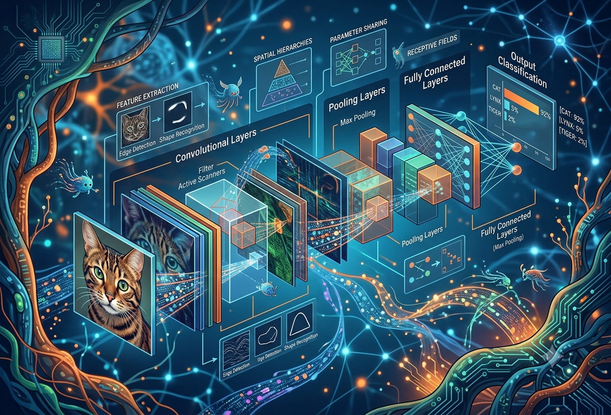
Convolutional Neural Networks (CNNs) — A Complete Reference Guide
What Is a Convolutional Neural Network?
A Convolutional Neural Network — usually written as CNN or ConvNet — is a special type of artificial intelligence that is extraordinarily good at understanding pictures, videos, and anything that has a spatial or grid-like structure.
A Convolutional Neural Network is a deep learning model that processes grid-structured data — most commonly images — by systematically scanning for visual patterns using mathematical operations called convolutions, stacking those learned patterns layer by layer until the model can recognise complex objects, scenes, and relationships.— utivra.com · AI Education Series
Think of it this way: when you look at a photograph of a cat, your eyes don’t examine the entire image all at once as one giant blob of information. Instead, your brain first picks out simple things — a curve here, a patch of fur colour there, pointy ear shapes — and then combines them into the whole concept of “cat.” A CNN does exactly the same thing, but with mathematics.
Imagine you are trying to find Waldo in a picture book. You don’t stare at the whole page at once — you move a small window across the page looking for Waldo’s striped shirt. A CNN does this too! It slides a tiny “inspection window” (called a filter) all across an image, looking for little clues. Then it puts all the clues together to figure out what the whole picture shows.
CNNs sit inside the broader family of Deep Learning models, which themselves are a subset of Machine Learning, which in turn is a branch of Artificial Intelligence. What makes CNNs special compared to ordinary neural networks is that they are purposely designed around the structure of images — they know that nearby pixels matter more to each other than far-away pixels, and they exploit this fact to work much more efficiently.
CNNs power the technology that unlocks your phone with your face, translates street signs in a foreign language through your camera, allows doctors to detect cancer in X-rays, and lets self-driving cars understand the road ahead. They have become one of the most transformative technologies in computing history.
Why CNNs Were Invented — The Problem They Solve
Before CNNs existed, teaching computers to understand images was painfully slow, expensive, and inaccurate. Understanding why those older methods failed explains exactly why CNNs are so clever.
The Old Approach: Fully-Connected Networks
The original solution for image recognition was to take every single pixel in a photo and feed it into a standard (fully-connected) neural network. Imagine a modest image — just 200 × 200 pixels with three colour channels (red, green, blue). That gives you 200 × 200 × 3 = 120,000 input numbers for a single image. If your first hidden layer has even 1,000 neurons, you immediately have 120,000 × 1,000 = 120 million parameters to learn. That is an enormous number — and most of them are redundant, because most pairs of pixels in an image simply don’t relate to each other.
Fully-connected networks treat every pixel as equally important to every other pixel. A pixel in the top-left corner of an image has zero mathematical relationship to a pixel in the bottom-right corner — and yet the old approach assumed they should influence each other. This wastes computation and makes it nearly impossible to learn efficiently from images.
Three Key Insights Behind CNNs
Features in images (edges, textures, shapes) emerge from small local neighbourhoods of pixels, not from pixels spread across the whole image. A CNN neuron only looks at a small patch at a time.
The same “edge detector” filter that finds a horizontal edge on the left of an image also works perfectly on the right side. CNNs reuse the same set of weights everywhere — this massively cuts the parameter count.
Simple patterns (edges, corners) are assembled into complex ones (textures, parts, objects) layer by layer, mirroring how the mammalian visual cortex is believed to work.
These three insights work together to produce a network that is both far more accurate on visual data and far more computationally efficient. A CNN for the same 200×200 image might only need a few million parameters instead of hundreds of millions — and it learns much better patterns in the process.
History & Key Milestones of CNNs
The story of CNNs stretches across four decades, weaving together neuroscience discoveries, mathematical breakthroughs, hardware revolutions, and vast new datasets.
Hubel & Wiesel — The Biological Blueprint
Neurobiologists David Hubel and Torsten Wiesel discovered that the cat’s visual cortex contains specialised neurons that respond only to specific orientations of lines. Certain neurons react to simple edges while others respond to more complex patterns — a hierarchy of visual processing. This Nobel Prize-winning work became the biological inspiration for CNNs.
Fukushima’s Neocognitron
Japanese researcher Kunihiko Fukushima built the Neocognitron — a hierarchical multi-layer network inspired directly by Hubel and Wiesel’s findings. It had separate “S-cells” (simple cells detecting features) and “C-cells” (complex cells combining them) — the conceptual forerunners of today’s convolutional and pooling layers.
Yann LeCun’s First Practical CNN
Yann LeCun at Bell Labs trained a CNN using backpropagation to recognise handwritten digits. This was the first time all the pieces — convolutional layers, shared weights, and gradient-based learning — were combined and demonstrated to work on a real problem.
LeNet-5 — The Gold Standard
LeCun published LeNet-5, an improved five-layer CNN that could reliably read handwritten zip codes and bank cheques. AT&T and major banks deployed it commercially — the first large-scale real-world CNN deployment in history.
AlexNet — The Deep Learning Revolution
Alex Krizhevsky, Ilya Sutskever, and Geoffrey Hinton unleashed AlexNet on the ImageNet Large Scale Visual Recognition Challenge (ILSVRC). It slashed the error rate from 26% to 15% — a margin so enormous it instantly convinced the entire research world that deep CNNs were the future of computer vision. This moment is widely considered the start of the modern AI boom.
VGGNet & GoogLeNet — Going Deeper
Oxford’s VGG group showed that simply making networks deeper (16–19 layers) with small 3×3 filters could dramatically improve accuracy. Simultaneously, Google’s Inception architecture introduced “inception modules” that processed filters of multiple sizes in parallel, winning ImageNet 2014.
ResNet — Solving the Vanishing Gradient
Microsoft Research’s Kaiming He introduced Residual Networks (ResNet) with 152 layers — achieving superhuman accuracy (3.57% error) on ImageNet. “Skip connections” allowed gradients to flow freely through extremely deep networks, solving the vanishing gradient problem that had previously made very deep CNNs untrainable.
MobileNets, EfficientNets & Beyond
Research shifted toward efficiency — building CNNs that could run on smartphones and embedded devices. MobileNet used “depthwise separable convolutions” to cut computation by 8–9×. EfficientNet introduced compound scaling to simultaneously balance depth, width, and image resolution. CNNs began merging with Transformer architectures in hybrid Vision Transformers (ViTs).
How CNNs See Images — Pixels, Channels & Volumes
Before we can understand what a CNN does, we need to understand how a computer stores and sees an image — because CNNs are designed precisely around that structure.
Images as Numbers
Every digital image is, at its core, a grid of tiny coloured squares called pixels. Each pixel has a colour, and that colour is stored as three numbers — the amount of Red, Green, and Blue light it contains — each ranging from 0 (none) to 255 (maximum). So a 1080×1920 HD photo is actually a cube of numbers: 1080 rows × 1920 columns × 3 colour channels.
In the language of deep learning, this 3D cube of numbers is called a tensor or a volume. The three dimensions are: width, height, and depth (where depth here means colour channels, not the number of layers in the network). CNNs are specifically designed to work with these 3D structures — preserving the spatial neighbourhood relationships between pixels as they process the data.
Researchers describe the shape of a volume as [Width × Height × Depth]. An HD image is 1920 × 1080 × 3. After passing through layers, this shape keeps changing — for example, after a convolution that produces 32 different feature maps it might become 1920 × 1080 × 32. Tracking these shape transformations is a key skill in CNN design.
The Convolutional Layer — Heart of the CNN
The convolutional layer is the defining innovation of a CNN. It is where raw pixel information is transformed into meaningful visual features through a scanning mathematical operation.
What Is Convolution?
Convolution is a mathematical operation where a small grid of numbers (called a filter or kernel) is slid across the input image. At each position, the filter’s numbers are multiplied with the image pixel values they are sitting on top of, and all those products are added together to produce a single output number. This process is repeated for every position across the image, generating a new grid of numbers called a feature map (or activation map).
Imagine you have a rubber stamp with a pattern on it. You press the stamp all over a piece of paper, moving it one step at a time — left to right, top to bottom. Each impression tells you how strongly that stamp’s pattern matches what’s on the paper at that spot. That is exactly what a CNN filter does to an image — it “stamps” across the entire picture, measuring how strongly a particular pattern (like a horizontal edge or a curved line) appears at every location.
Key Parameters of a Convolutional Layer
A CNN layer uses many filters simultaneously — perhaps 32, 64, or 512. Each filter specialises in detecting a different type of pattern. Early filters learn simple things like horizontal edges, vertical edges, and diagonal lines. Deeper filters learn complex patterns like textures, object parts, and eventually entire objects. Critically, the filter weights are not hand-coded by humans — they are learned automatically through training on thousands of example images.
Stride controls how far the filter jumps between positions. A stride of 1 means the filter moves one pixel at a time (producing a large output map). A stride of 2 means it jumps two pixels (producing a roughly half-sized output map). Larger strides reduce computation and output size but can miss fine-grained patterns.
When a filter slides to the edge of an image, it would normally shrink the output size. Zero-padding adds a border of zeros around the image so the output remains the same size as the input (“same padding”). Without padding (“valid padding”), the output shrinks with each convolution.
The receptive field of a neuron is the region of the input image that influences its output. In early layers, each neuron’s receptive field is small (e.g. 3×3 pixels). In deeper layers, because each layer builds on the previous one, a single neuron’s receptive field can span the entire image — allowing the network to make sense of global context.
One filter has, say, 3×3×3 = 27 weights (+1 bias = 28 parameters). That same filter is reused at every position in the image. So instead of millions of independent weights, the entire layer might only have 28 × 32 = 896 parameters. This parameter sharing is why CNNs are so much more efficient than fully-connected networks on image data.
The Pooling Layer — Shrinking Smartly
After a convolutional layer creates detailed feature maps, a pooling layer steps in to intelligently compress them — keeping the important information while throwing away spatial noise and reducing the computation needed for all subsequent layers.
What Does Pooling Do?
Pooling is a downsampling operation. It divides the feature map into small, non-overlapping rectangular regions and replaces each region with a single representative value. The most common variant is Max Pooling, which takes the largest value from each region. The idea is that if a feature (like an eye in a face) is detected somewhere in a region, the exact pixel location matters less than the fact that it was found there at all.
Types of Pooling
Keeps the largest value from each region. Best at preserving sharp, high-contrast features like edges. The dominant choice in most CNN architectures.
Computes the mean of all values in each region. Produces smoother, more evenly distributed feature maps. Sometimes used in the final layers of a network.
Collapses an entire feature map into a single number (the average of all values). Used in modern architectures like ResNet to replace the flat fully-connected layers, drastically reducing parameters.
Pooling layers have no learnable parameters — they simply apply a fixed mathematical operation. Their benefits are threefold: they reduce spatial dimensions (cutting computation), introduce a degree of translation invariance (the CNN can recognise a cat even if it is slightly shifted in the image), and help prevent overfitting.
Activation Functions — Teaching the Network to Think Non-Linearly
A CNN composed only of convolutions and matrix multiplications would just be a glorified linear equation — and linear equations cannot distinguish a cat from a dog no matter how large they get. Activation functions inject the non-linearity that allows CNNs to learn complex, multi-layered patterns.
After every convolution, the network applies an activation function element-wise to every single value in the feature map. This decides whether and how strongly each neuron “fires” — whether the pattern that filter detected is strong enough to matter.
| Activation | Formula | Output Range | When Used | Key Advantage |
|---|---|---|---|---|
| ReLU | max(0, x) | [0, ∞) | After most conv layers | Extremely fast; combats vanishing gradients |
| Leaky ReLU | max(0.01x, x) | (−∞, ∞) | When ReLU causes “dead neurons” | Allows small gradient for negative inputs |
| Sigmoid | 1/(1+e⁻ˣ) | (0, 1) | Binary output layer | Maps to probability directly |
| Softmax | eˣⁱ / Σeˣ | (0, 1) summing to 1 | Multi-class final layer | Converts scores to class probabilities |
| GELU | x·Φ(x) | (−0.17, ∞) | Modern transformers & CNNs | Smooth gradient; excellent performance |
ReLU (Rectified Linear Unit) — simply “set negative values to zero, keep positive values unchanged” — became the default choice for CNN hidden layers around 2012 and remains dominant. It is almost absurdly simple, but it solves the devastating vanishing gradient problem that made training deep networks nearly impossible with older activations like tanh or sigmoid. When gradients pass through dozens of layers during backpropagation, older activations squeeze them toward zero; ReLU does not.
Imagine a light switch that doesn’t just turn on and off, but dims in proportion to how much light you want. ReLU is like a switch that ignores all darkness (negative values go to zero) but passes through all light exactly as bright as it came in. This simple rule prevents signal from getting lost as it travels through dozens of layers.
The Fully-Connected Layer — Making the Final Decision
After the convolutional and pooling layers have extracted rich, hierarchical visual features from the image, one or more fully-connected layers take those features and combine them into a final classification decision.
At this stage, the 3D feature maps produced by the final pooling layer are flattened into a single long vector of numbers. This vector is then fed into a standard fully-connected (dense) neural network layer — every neuron in the layer receives every value from this vector. The fully-connected layers learn high-level reasoning: “if there are pointy ear features AND whisker features AND fur texture features in the right spatial arrangement, the answer is ‘cat.'”
The very last fully-connected layer produces one output number per class (e.g. 1000 output neurons for a network trained on 1000 different categories). A Softmax activation function converts these raw scores into probabilities that add up to 100%, and the class with the highest probability is the network’s prediction.
Many modern architectures (like ResNet, MobileNet, and EfficientNet) replace the large fully-connected layers with Global Average Pooling — which collapses each feature map to a single number. This removes millions of parameters, reduces overfitting, and allows the network to accept images of any size. The final fully-connected layer for classification is then applied to this tiny averaged vector instead of a massive flattened one.
The Full CNN Architecture — All Layers Together
Now we can see how all the pieces fit together into a complete pipeline that transforms a raw image into a confident prediction.
The key pattern to notice is that as we go deeper into the network, the spatial dimensions (width and height) of the feature maps shrink (due to pooling), while the number of feature maps (depth/channels) grows. Early layers produce many large maps describing low-level features; deep layers produce fewer but smaller maps describing high-level abstract features. The fully-connected layers at the end collapse this entire information structure into a final classification verdict.
How CNNs Learn — Training with Backpropagation
A newly created CNN knows absolutely nothing — its filters contain random numbers, producing meaningless outputs. Training is the process of showing it thousands of labelled examples and gradually adjusting every weight until its predictions become accurate.
The Training Loop
Loss Functions
A loss function measures how far the CNN’s prediction is from the correct answer. For image classification, Cross-Entropy Loss is standard — it penalises the network heavily when it is confident but wrong, and less so when it is uncertain. For object detection or image segmentation tasks, different loss functions are used that account for spatial accuracy.
Optimisers — How Weights Are Updated
The foundational optimiser. Updates weights by moving in the direction that reduces loss, one mini-batch at a time. Requires careful tuning of the learning rate.
Adapts the learning rate automatically for each weight using estimates of first and second-order gradient moments. Much easier to tune than SGD; the current default for most CNN training.
Keeps a running average of squared gradients to normalise updates. Historically important for recurrent networks; still occasionally used for CNNs.
Regularisation — Preventing Overfitting
A CNN can memorise its training set without learning anything general — this is called overfitting. Several techniques fight this:
- Dropout — randomly deactivates a fraction (typically 50%) of neurons during each training step, forcing the network to build redundant, robust representations rather than relying on any single pathway.
- Batch Normalisation — normalises the activations within each mini-batch during training, stabilising learning and allowing much higher learning rates. This has become nearly universal in modern CNNs.
- Data Augmentation — artificially expands the training set by applying random flips, rotations, crops, colour jitter, and other transformations to existing images. The CNN sees slightly different versions of each image every epoch, making it harder to memorise and better at generalising.
- L2 Regularisation (Weight Decay) — adds a penalty for large weights to the loss function, discouraging the network from placing too much importance on any single connection.
Training a CNN is like studying for an exam. If you only ever read the same ten questions (training data without augmentation), you might memorise the exact wording without understanding the concept. But if your teacher keeps rephrasing the questions slightly (data augmentation), and occasionally covers some of your notes (dropout), you build genuine understanding that works even on questions you have never seen before.
Famous CNN Architectures
Over the past decade, a series of influential CNN architectures has shaped the field. Each one solved a specific problem or introduced an innovation that all subsequent networks borrowed from.
Layers: 5 (2 Conv + 3 FC) · Parameters: ~60K · Input: 32×32 grayscale. The pioneer. Deployed commercially for cheque reading. Established the CONV → POOL → CONV → POOL → FC pattern that every subsequent architecture followed.
Layers: 8 (5 Conv + 3 FC) · Parameters: ~60M · Input: 224×224 RGB. Used ReLU activations, dropout, and data augmentation — all novel at scale. Trained on 2 GPUs. Won ImageNet 2012 by a historic margin and ignited the deep learning revolution.
Layers: 16 or 19 · Parameters: ~138M · Input: 224×224. Oxford’s team proved that depth matters — using only tiny 3×3 filters but stacking many more layers. The two stacked 3×3 filters have the same effective receptive field as one 5×5 filter but fewer parameters. Widely used as a feature extractor backbone.
Layers: 22 · Parameters: ~7M (!) · Input: 224×224. Introduced “Inception modules” — blocks that process 1×1, 3×3, and 5×5 convolutions in parallel, then concatenate results. Auxiliary classifiers injected gradients mid-network. Won ImageNet 2014 with 7× fewer parameters than AlexNet.
Layers: 18 to 152 · Parameters: ~25M (ResNet-50) · Input: 224×224. Introduced “skip connections” (residual connections) that let gradients bypass layers, enabling training of extremely deep networks without vanishing gradients. ResNet-50 is arguably the most widely used backbone in all of computer vision today.
Layers: 28 · Parameters: ~4M · Input: 224×224. Designed for mobile and embedded devices. Replaced standard convolutions with “depthwise separable convolutions” — splitting a single convolution into two cheaper operations, cutting computation by 8–9×. Runs in real-time on smartphones.
Layers: Variable · Parameters: 5.3M (B0) to 66M (B7). Google Brain’s systematic approach to scaling: simultaneously scale depth, width, and resolution by a fixed compound factor. EfficientNet-B7 surpassed all previous models on ImageNet with far fewer parameters.
Layers: Variable · Parameters: ~29M (Tiny). “Modernised” the pure CNN by incorporating design ideas from Vision Transformers — larger kernels (7×7), depthwise convolutions, fewer activation functions, layer normalisation instead of batch normalisation. Competitive with ViTs while retaining CNN simplicity.
Each great CNN architecture solved one specific bottleneck — depth, width, efficiency, or training stability — and every solution became a building block adopted by every architecture that followed.
— utivra.com · AI Education SeriesWhere CNNs Are Used — Real-World Applications
CNNs have moved from academic curiosity to mission-critical infrastructure across nearly every industry. Here is where they are making a difference right now.
Healthcare & Medical Imaging
CNNs examine X-rays, MRI scans, CT scans, and pathology slides to detect cancer, fractures, diabetic retinopathy, and skin lesions — often matching or exceeding specialist radiologist accuracy. Google’s DeepMind detected over 50 eye diseases from retinal scans with 94% accuracy. Faster screening means earlier intervention and saved lives.
Autonomous Vehicles
Self-driving cars process dozens of camera feeds simultaneously using CNN-based systems to detect pedestrians, other vehicles, traffic signs, lane markings, and obstacles in real time. Companies like Tesla, Waymo, and Mobileye rely on CNNs as the core perception layer of their autonomous driving stacks.
Face Recognition & Security
Your phone’s Face ID uses a CNN trained on thousands of facial features to verify your identity in milliseconds. CNNs power surveillance systems, airport boarding gates, payment authorisation (Alipay, Apple Pay), and social media auto-tagging. They can identify a face in a crowded scene even in partial occlusion or poor lighting.
Agriculture & Food
Drones equipped with CNNs survey fields and identify crop diseases, pest damage, and nutrient deficiencies from aerial images — before they are visible to the human eye. Supermarkets deploy CNNs to monitor freshness of produce on shelves. Quality control systems use CNNs to spot defects in packaged foods.
Manufacturing & Quality Control
Factory assembly lines use CNN-powered cameras to inspect products for surface defects, misalignments, and component errors at speeds impossible for human inspectors. Semiconductor manufacturers use CNNs to identify microscopic chip defects. This has dramatically reduced manufacturing waste and recall rates.
Satellite & Geospatial Imaging
CNNs analyse satellite imagery to map deforestation in real-time, monitor illegal construction, track shipping traffic, estimate solar panel output from rooftop photos, and predict crop yields globally. Governments and NGOs use these systems to enforce environmental law and plan disaster response.
Creative AI & Content Generation
CNNs power style transfer (applying Van Gogh’s painting style to your photo), image super-resolution (making low-resolution images sharp), photo restoration, and real-time image filters in apps. The visual understanding components of text-to-image models like Stable Diffusion and DALL·E are also rooted in convolutional principles.
Scientific Research
Astronomers use CNNs to classify galaxies from telescope images and detect gravitational lensing. Particle physicists at CERN use them to identify collision events in detector data. Biologists use CNN-based tools to analyse microscopy images of cells and identify protein structures.
Pros & Cons of Convolutional Neural Networks
CNNs are extraordinarily powerful for visual tasks — but like every technology, they come with real limitations that practitioners must understand.
✓ Strengths
- Unmatched visual accuracy — CNNs consistently achieve state-of-the-art results on image classification, detection, and segmentation benchmarks, often surpassing human-level performance on narrow tasks.
- Automatic feature learning — no human expert needs to manually engineer features. The network discovers the most useful representations on its own during training.
- Translation invariance — because of pooling and parameter sharing, CNNs can recognise an object regardless of where it appears in an image.
- Parameter efficiency — weight sharing means far fewer parameters than a fully-connected network of equivalent capacity, making training and deployment more manageable.
- Transfer learning — a CNN trained on millions of images can be fine-tuned for a new task with just thousands of examples, drastically reducing training time and data requirements.
- Interpretable intermediate representations — feature maps can be visualised, giving researchers insight into what patterns each layer has learned — unlike some other ML methods.
- Hardware-optimised — GPU architectures are specifically designed for the matrix operations CNNs use, enabling fast training and inference at scale.
✗ Limitations
- Data hunger — training a CNN from scratch typically requires tens of thousands to millions of labelled examples. Collecting and annotating this data is expensive and time-consuming.
- Computational cost — large CNNs require significant GPU resources and memory for both training and inference, which can be prohibitive for smaller organisations or edge deployments.
- Poor global reasoning — standard CNNs are locally focused by design. They can struggle with tasks requiring long-range spatial relationships across the entire image — an area where Vision Transformers have an advantage.
- Adversarial vulnerability — a CNN can be fooled by subtly altered images (adversarial examples) that are completely indistinguishable to a human but cause dramatic misclassification.
- Black-box nature — while feature maps give some interpretability, it is still difficult to fully explain precisely why a CNN made a specific decision — a problem in high-stakes medical or legal contexts.
- Assumes spatial structure — CNNs are specifically designed for grid-structured data. Applying them to non-spatial data (text, graphs, audio) requires careful adaptation and may not be the best tool.
- Inductive biases limit flexibility — the local connectivity assumption that makes CNNs efficient on images can be a constraint when working with data that lacks clear spatial locality.
Researchers have shown that adding a tiny, carefully calculated noise pattern to an image — invisible to human eyes — can cause a CNN to misclassify a clearly correct image with extreme confidence. A panda can become a gibbon. A stop sign can be misread as a speed limit sign. This vulnerability is a critical challenge for safety-critical deployments like self-driving cars, and it reveals that CNNs learn statistical patterns rather than true conceptual understanding of the world.
The Future of CNNs — What Comes Next?
CNNs are not standing still. The field is evolving rapidly — merging with transformer architectures, becoming more efficient, and expanding beyond vision into entirely new domains.
Vision Transformers (ViTs) excel at global reasoning while CNNs excel at local feature extraction. Hybrid architectures like CoAtNet and ConvNeXt-V2 combine both strengths — CNN-style early layers feed into transformer-style attention layers for global context.
Neural Architecture Search (NAS) automates the design of compact, fast CNNs tailored to specific hardware — enabling real-time inference on microcontrollers and IoT devices with milliwatt power budgets.
Researchers are developing techniques to make CNNs resistant to adversarial attacks, more calibrated in their uncertainty, and better at communicating why they reached a decision — essential for medical and autonomous systems.
Extending convolution to 3D (processing video as a spatial + temporal volume) enables action recognition, medical volumetric analysis (3D MRI/CT), and point-cloud processing for autonomous vehicles and robotics.
From predicting protein folding from microscopy images to detecting gravitational waves in telescope data, CNNs are becoming standard tools in scientific discovery — wherever large datasets of structured observations need automated analysis.
New training paradigms (DINO, SimCLR, MAE) allow CNNs to learn powerful representations from unlabelled images by predicting masked patches or matching augmented views — reducing the dependency on expensive human annotations.
CNNs were the proof of concept that deep, hierarchical feature learning works. The principles they established — local connectivity, parameter sharing, learned representations — remain the foundation of modern computer vision even as architectures evolve far beyond the original design.— utivra.com · AI Education Series
The story of convolutional neural networks is, in many ways, the story of modern artificial intelligence itself. From a biological inspiration in a cat’s visual cortex in 1959, through decades of limited hardware and skepticism, to the ImageNet revolution of 2012 that convinced the world that deep learning was real — CNNs demonstrated that machines could learn to perceive the world with astonishing fidelity. The architectures will keep evolving, the applications will keep expanding, and the fundamental insight — that visual understanding emerges from hierarchical, local, shared feature detection — will endure.
Sources & References
Foundational tutorial covering CNN basics, layer types, and working principles.
Enterprise-focused explainer on CNN structure, applications, and deployment considerations.
Interactive textbook with executable code and mathematical derivations of CNN concepts.
Practical guide oriented toward data labelling and training pipelines.
Cloud-perspective overview of CNN use cases and deployment patterns.
The canonical academic reference for CNN architecture and mathematical foundations.
Hardware-aware perspective on CNN computation and GPU acceleration.
Comprehensive encyclopaedic reference with history, variants, and citations.
Engineering and applied mathematics perspective on CNN design and training.
Computer-vision practitioner’s guide with code examples and visual explanations.
Peer-reviewed academic research context and engineering applications of CNNs.
Enterprise IT perspective on CNN deployment, benefits, and limitations.